El e c t ro n ic
Jo ur n
a l o
f P
r o b
a b i l i t y
Vol. 13 (2008), Paper no. 18, pages 530–565. Journal URL
http://www.math.washington.edu/~ejpecp/
Bounding a Random Environment
for Two-dimensional Edge-reinforced Random Walk
Franz Merkl Mathematical Institute
University of Munich
Theresienstr. 39, D-80333 Munich, Germany
Email: [email protected]
http://www.mathematik.uni-muenchen.de/~merkl
Silke W.W. Rolles
Zentrum Mathematik, Bereich M5, Technische Universit¨at M¨unchen D-85747 Garching bei M¨unchen, Germany
Email: [email protected]
http://www-m5.ma.tum.de/pers/srolles
Abstract
We consider edge-reinforced random walk on the infinite two-dimensional lattice. The process has the same distribution as a random walk in a certain strongly dependent random envi-ronment, which can be described by random weights on the edges. In this paper, we show some decay properties of these random weights. Using these estimates, we derive bounds for some hitting probabilities of the edge-reinforced random walk .
Key words: Reinforced random walk, random environment.
1
Introduction
Definition of the model. Linearly edge-reinforced random walk (ERRW) on Z2 is the fol-lowing model: Consider the two-dimensional integer latticeZ2 as a graph with edge set
E={{x, y} ∈Z2×Z2 : |x−y|= 1}. (1.1) Here, | · | denotes the Euclidean norm. In particular, the edges are undirected. Fix a vertex
v0 ∈ Z2 and a positive number a > 0. A non-Markovian random walker starts in X0 = v0.
At every discrete time t ∈ N0, it jumps from its current position Xt to a neighboring vertex
Xt+1 in Z2, |Xt+1 −Xt| = 1. The law Pv0,a of the random walker is defined in terms of the
time-dependent weights
we(t) =a+ t−1
X
s=0
1{e={Xs,Xs+1}}, e∈E. (1.2)
The weight we(t) of edge eat time tequals the number of traversals ofe up to timet plus the initial weight a. Thus, we(t) increases linearly in the number of crossings of e. The transition probabilityPv0,a[{Xt, Xt+1}=e|X0, . . . , Xt] is proportional towe(t) for all edgese∋Xt:
Pv0,a[{Xt, Xt+1}=e|X0, . . . , Xt] =
we(t) P
e′∋Xtwe′(t)1{e∋Xt}. (1.3)
This model was introduced by Diaconis [Dia88]. Throughout this paper, “edge-reinforced random walk” will always mean “linearly edge-reinforced random walk”, as defined above. We do not consider any other reinforcement scheme.
Main open problem and previous results forZd. As Pemantle [Pem88] remarks, Diaconis asked whether this process onZ2 and more generally on Zd, d≥2, is recurrent. This question is still open almost twenty years after it was raised. Even worse, provinganything about edge-reinforced random walk onZ2tends to be hard. To our best knowledge, almost nothing is known about edge-reinforced random walk on Zdfor anyd≥2, with only a few exceptions:
1. Sellke [Sel94] has proved for edge-reinforced random walk on Zdin any dimension d, that almost surely the range is infinite, and that the random walker hits each coordinate plane
xk= 0, k= 1, . . . , dalmost surely infinitely often.
2. Recently, in [MR07c], we have shown that the edge-reinforced random walk on any locally finite graph has the same distribution as a random walk in a random environment given by random, time-independent, strictly positive weights (xe)eon the edges. As a consequence, the edge-reinforced random walk on any infinite, locally finite, connected graph visits all vertices infinitely often with probability one if and only if it returns to its starting point almost surely.
does not stay very close to its starting point. Rather, the random walker spends most of its time at some, possibly infinitely many, small islands located at varying distance from the starting point. This indicates that the weights (xe)ein (b) might vary in rather small regions over many orders of magnitude.
Intention of this paper. In this paper, we show for an edge-reinforced random walk on Z2
that at least in a weak, stochastic sense, the weightsxe in (b) converge to 0 asegets infinitely far from the origin. This provides the first analysis of the global behaviour of the random environment over Z2. Bounds on the weights xe induce information for the law of the edge-reinforced random walk. For example, our bounds allow for the first time the estimation of hitting probabilities of the paths of edge-reinforced random walk onZ2.
The present paper is independent of our papers [MR07a], [MR05], [Rol06] on edge-reinforced random walk on ladders, as the transfer operator technique used there breaks down in two dimensions.
Previous results on other graphs. For graphs where the edge-reinforced random walk is recurrent, a representation different from the one in [MR07c] follows from the paper [DF80] by Diaconis and Freedman, which was written before edge-reinforced random walk was introduced. For finite graphs, Coppersmith and Diaconis [CD86] discovered an explicit, but complicated formula for the joint law of the fraction of time spent on the edges. In fact, this joint law just equals the law of the weights (xe)enormalized appropriately; see [Rol03]. A proof of the formula describing the joint law of (xe)e is published in [KR00]. The random environment is strongly dependent, unless the graph is a tree-graph.
Pemantle [Pem88] examined the model on infinite trees; in particular, he showed that the pro-cess on tree graphs has the same distribution as a random walk in an independent random environment.
On infinite ladders, for sufficiently large initial weights a, the random environment can be de-scribed as an infinite-volume Gibbs measure. It arises as an infinite-volume limit of finite-volume Gibbs measures; see [MR05], [Rol06], [MR07a]. The finite-volume Gibbs measures are just a reinterpretation of the formula of Coppersmith and Diaconis in the version described by Keane and Rolles. This reinterpretation has been used in the above references to prove recurrence of the process on ladders and also to analyze the asymptotic behavior of the edge-reinforced random walk in more detail.
In [MR07b], we have recently proven recurrence of the edge-reinforced random walk on some fully two-dimensional graphs different fromZ2. In the present paper, we push the method used for these graphs to its limits: Unlike in [MR07b], in the present paper, we prove bounds for the random weights in infinite volume, and we prove strong bounds for the expected logarithm of the random weights. These bounds require more sophisticated deformations than in [MR07b]. However, the present paper can be read independently of [MR07b].
2
Results
We present results for edge-reinforced random walk onZ2 (“infinite volume”), but also on finite boxes inZ2 with periodic boundary conditions (“finite volume”). The latter results are used in the proof of the former ones.
All constants likeβ(a), c1, c2, . . . keep their meaning throughout the whole article.
2.1 Hitting probabilities for ERRW
For v ∈ Z2, let τv := inf{n≥ 1 :Xn = v} denote the first time ≥ 1 when the random walker visitsv.
Theorem 2.1(Hitting probabilities for ERRW). For alla >0, there arec1(a)>0andβ(a)>0,
such that for all v∈Z2\ {0}, the following hold:
1. The probability to reach the vertex v before returning to the vertex 0 is bounded by
P0,a[τv < τ0]≤c1(a)|v|−β(a). (2.1)
2. For alln≥1, the probability that the random walker visits the vertexv at timen satisfies the same bound
P0,a[Xn=v]≤c1(a)|v|−β(a). (2.2)
Although these estimates are weak if compared with what is known forsimple random walk on
Z2, to our knowledge, no bounds of any similar type were known before.
If we knew β(a) >1, the estimate (2.1) would imply recurrence. However, our estimates yield only
β(a) =£
1024e(1 + 4a)(1 + (e·max{⌈1/√a⌉,2}log 2)−1)¤−1. (2.3)
In particular,β(a) is a decreasing function of awith
β(a)a−→→0 1
1024e and β(a)
a→∞
−→ 0. (2.4)
Thus recurrence is still an open problem. Furthermore, our estimates yield
c1(a) = 2·(6
√
2 max{⌈1/√a⌉,2})β(a). (2.5)
This fulfills
2.2 Bounds in infinite volume
Set Ω = (0,∞)E. For x∈Ω, let Qv0,x denote the law of a Markovian nearest neighbor random
walk on (Z2, E) with starting point v0 in a time-independent environment given by the edge
weightsx. Given this random walk is atuand given the past of the random walk, the probability it jumps to the neighboring vertex v is proportional to the weightxe of the edgee={u, v}. Edge-reinforced random walk onZ2 can be represented as a random walk in a random environ-ment (RWRE). More precisely:
Theorem 2.2 (ERRW as RWRE, Theorem 2.2 in [MR07c]). Let a >0. There is a probability measureQ0,a onΩ, such that for all events A⊆(Z2)N0, one has
P0,a[A] = Z
Ω
Q0,x[A]Q0,a(dx). (2.7)
It is not known whetherQ0,a is unique up to normalization of the edge weightsx. In this article, we prove some decay properties of the random environment. These results hold for at least one choice ofQ0,a. Forx∈Ω andv∈Z2, set
xv = X
e∋v
xe. (2.8)
The following two theorems show that in some weak probabilistic sense, the ratios of weights
xv/x0 tend to zero as |v| → ∞. We phrase two formal versions of this statement. The first
version only cares about the expected logarithms of ratiosxv/x0. In this version, we get a fast
divergence to −∞as|v| → ∞if only a >0 is small enough.
Theorem 2.3 (Decay of the expected log weights). There exist functions c2, c3:
(0,∞) →(0,∞) with c2(a) → ∞ as a↓ 0, such that the following holds: For all a >0 and all v∈Z2\ {0},
EQ0,a
·
logxv
x0
¸
≤c3(a)−c2(a) log|v|. (2.9)
Such a fast decay of the logarithms of the weights in a stochastic sense has not been proven before onanyfully two-dimensional graph. The methods used in [MR07b] do not suffice to prove such a bound.
However, Theorem 2.3 does not imply weak convergence of xv/x0 to zero. Weak convergence is stated among others in the following theorem, but our bound for the rate of convergence is not as strong as in the preceding theorem.
Theorem 2.4(Decay of the expected weight power). For alla >0, there are constantsc1(a)>0
and β(a)>0, such that for all v∈Z2\ {0}, the following holds:
EQ0,a
"µ
xv
x0
¶14#
≤c1(a)|v|−β(a). (2.10)
The estimates for the hitting probabilities of the edge-reinforced random walk in Theorem 2.1 are derived from the bounds in the preceding theorem.
Let e, f ∈ E be two neighboring edges, i.e. two edges containing a common vertex v. The random variables log(xe/xf) with respect to Q0,a are tight with exponential tails, uniformly in the choice of the edgeseand f. This is stated formally in the following theorem:
Theorem 2.5 (Tightness of ratios of neighboring edge weights). For all a > 0 and all α ∈
(0, a/2), one has
sup e,f∈E e∩f6=∅
EQ0,a
·µ
xe
xf ¶α¸
<∞. (2.11)
2.3 Uniform bounds in finite volume
All our infinite-volume results are derived from uniform finite-volume analogs for edge-reinforced random walk on finite boxes. “Uniform” here means “uniform in the size of the finite box”. We consider a (2N+ 1)×(2N + 1) box
V(N)=Z2/(2N + 1)Z2 (2.12)
with periodic boundary conditions. Forv∈Z2, let v(N)=v+ (2N+ 1)Z2 denote the class of v
inV(N). If there is no risk of confusion, we identifyV(N)with the subset ˜V(N)= [−N, N]2∩Z2
ofZ2. Let
E(N) ={{u(N), v(N)}: {u, v} ∈E}. (2.13) For an equivalence class v(N) =v+ (2N+ 1)Z2, set
¯ ¯ ¯v
(N)¯¯
¯= min{|v+ (2N+ 1)z|: z∈Z
2
}. (2.14)
This is just the Euclidean distance ofv(N) to the origin, viewed as an element of ˜V(N).
Just as in the infinite-volume case, for v0 ∈ V(N) and a >0, let Pv(0N,a) denote the law of
edge-reinforced random walk on (V(N), E(N)) with starting pointv0and constant initial weightsa. Set
Ω(N)= (0,∞)E(N). Forx∈Ω(N), letQ(vN0,x) denote the law of a random walk on (V(N), E(N)) with
starting pointv0 in a time-independent environment given by weightsx. Note that multiplying
all components of x by the same (possibly x-dependent) scaling factor α does not change the law of the corresponding random walk. The following finite-volume analog of Theorem 2.2 is well-known:
Theorem 2.6 (ERRW as RWRE on finite boxes, Theorem 3.1 in [Rol03]).
Let a >0 and v0 ∈V(N). There is a probability measure Q(vN0,a) onΩ(N), such that for all events
A⊆(V(N))N0, one has
Pv(0N,a)[A] =
Z
Ω(N)
Q(vN0,x)[A]Q(vN)
0,a(dx). (2.15)
Up to an arbitrary normalization of the random edge weights x ∈ Ω(N), the law Q(vN0,a) of the
In [Dia88] and [KR00], the distributionQ(vN0,a) is described explicitly; see also Lemma 4.1, below. The weaker statement that the edge-reinforced random walk on (V(N), E(N)) is a mixture of Markov chains follows already from [DF80].
The following two theorems are finite-volume analogs of Theorems 2.3 and 2.4. The bounds are uniform in the size of a finite box.
Theorem 2.7 (Decay of the expected log weights in finite volume). There exist
functions c2, c3 : (0,∞) → (0,∞) with c2(a) → ∞ as a↓ 0, such that the following holds: For
Theorem 2.8 (Decay of the expected weight power in finite volume). For all initial weights
a > 0, there are c1(a) >0 and β(a) >0, such that for all N ∈N and all v ∈ V(N)\ {0}, the
The analog of Theorem 2.5 holds also in finite volume, uniformly in the sizeN of the box: Lemma 2.9. For all a >0 and all α∈(0, a/2), one has
3
The big picture – intuitively explained
The main work in the paper consists of showing the bounds of Theorems 2.7 and 2.8, which concern finite boxes. Before giving detailed proofs, let us first explain roughly and informally the ideas coming from statistical mechanics. The purpose of this section is only to give an overview and some intuitive picture. Detailed proofs are given in Sections 4–8; they can be checked even when one ignores this intuition completely.
We start Section 4 by reviewing an explicit description of the mixing measureQ(vN0,a) from equation (2.15), (Lemma 4.1, below). For two different starting points 0 andℓof the random walk paths, the mixing measures are mutually absolutely continuous with the Radon-Nikodym derivative
We interpolate betweenQ(0N,a) andQ(ℓ,aN) by an exponential family, in other words, by a family of Gibbs distributions
dPη = 1
Zη
eηΣℓdQ(N)
0,a , 0≤η≤1 ((4.9) below) (3.2)
with a normalizing constant (partition sum) Zη = EQ(N) 0,a
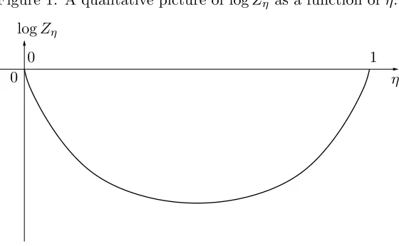
[exp(ηΣℓ)]. By symmetry considera-tions, one knowsZη =Z1−η andEPη[Σℓ] =−EP1−η[Σℓ]; see Figure 1 and formula (8.10), below.
Note that
d
dηlogZη =EPη[Σℓ] and
d2
dη2logZη = VarPη(Σℓ). (3.3)
Figure 1: A qualitative picture of logZη as a function ofη. logZη
η
0 0
1
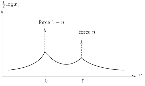
In the language of statistical physics, the random environment described byPη may be imagined as a rubber membrane, exposed to thermal fluctuations. For a vertexv, 12logxv is interpreted as the height of the membrane at the locationv; thus Σℓ = 12(logxℓ−logx0) gets the interpretation
of a height difference.
Figure 2: An intuitive picture for a rubber membrane described byPη
v 1
2logxv
force 1−η
forceη
0 ℓ
We are interested in the elastic properties of the rubber membrane:
• On the one hand, this involves how much the expected height differenceEPη[Σℓ] changes as
the forceηvaries from 0 to 1. Indeed, the expected logarithm in (2.16) can be interpreted in terms of this change:
EQ(N) 0,a
·
logxℓ
x0
¸
= 2EP0[Σℓ] =−2EP1[Σℓ] =EP0[Σℓ]−EP1[Σℓ]. (3.4)
• On the other hand, it also involves the physical work (change of the free energy, where the free energy is given by−logZη) acting on the membrane as the forceη varies from 1/2 to 0. Indeed, the logarithm of the quantity bounded in (2.17) gets the interpretation of this physical work:
logE
Q(0N,a)
" µ
xℓ
x0
¶1/4#
= logZ1/2= logZ1/2−logZ0. (3.5)
Both items can be bounded by the same method (Section 6), using a general variational principle for free energies. Let us first explain this variational principle abstractly: Consider two mutually absolutely continuous probability measures, a reference measure σ and a thermal measure µ, where
dµ= 1
Ze
−βHdσ (3.6)
with a HamiltonianH, a temperatureT =β−1, and the normalizing constant
Z =Eσ[e−βH] = 1
Eµ[eβH]
. (3.7)
For probability measuresν, define the free energy
with the internal energyU(ν) =Eν[H] and the entropy (with the sign convention used in physics)
S(ν, σ) =−Eν[log(dν/dσ)], whenever these quantities exist. Then the functionalν7→F(ν, σ) is minimized forν =µ, with the minimumF(µ, σ) =−β−1logZ. Indeed,
F(ν, σ)−F(µ, σ) =−β−1S(ν, µ)≥0. (3.9)
We apply this variational principle for σ = Pη, µ = Q(0N,a), β = η, H = Σℓ, and Z = Zη−1. In Subsection 5.2, we take some “deformed measure”ν = Πγ,η ((5.13), below) of σ, with a deformation parameterγ. The deformed measure ν is intended to be close to µ. The physical picture of the rubber membrane exposed to external forces motivates us to define the deformed measureν, using a deformation map Ξγ(Definition 5.5, below), which changes the heights of the membrane approximately proportional to the Green’s function of the Laplace operator in two dimensions (Definitions 5.2 and 5.3, below). With the right choices, the internal energy changes linearlyin the deformation parameter,
U(ν)−U(σ) = const·γ (expectation of (6.5), below), (3.10)
while the the entropy fulfills a quadraticbound
−S(ν, σ)≤const(ℓ)·γ2 ((5.15), below), (3.11)
as it has a minimum atγ = 0.
The proof of this entropy bound with good estimates for the constant const(ℓ) is technically involved (Subsection 5.2). We have much better bounds for the constant const(ℓ) in the case
η = 1 than for all other values of η, since P1 is much easier to control than general Pη; this is the main obstruction against an answer to Diaconis’ recurrence question.
By the variational principle, we arrive at
η−1logZη =−β−1logZ =F(µ, σ) ≤F(ν, σ) =U(ν)−η−1S(ν, σ)
≤U(σ) + const·γ+ const(ℓ)η−1γ2=EPη[Σℓ] + const·γ+ const(ℓ)η
−1γ2. (3.12)
Optimizing overγ yields the key estimate (Theorem 6.1 below)
logZη−ηEPη[Σℓ]≤ −const
′(ℓ)
·η2. (3.13)
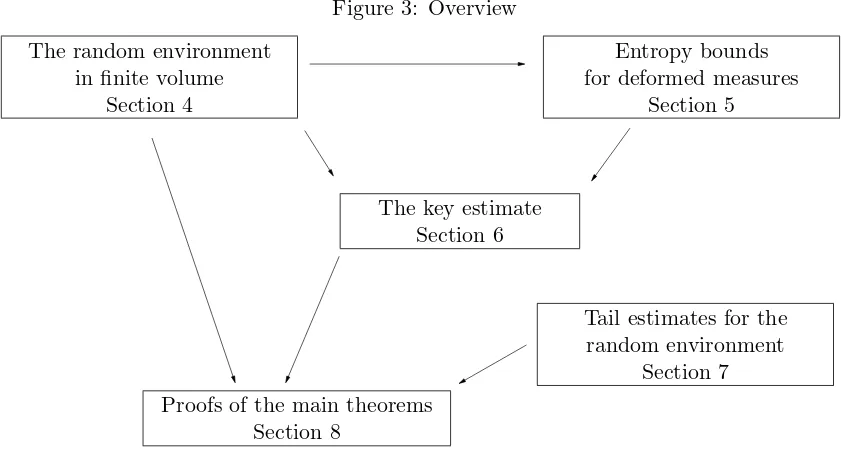
In the special cases η = 1 and η = 1/2, this yields the bounds for the expectations in (3.4) and (3.5) as claimed in Theorems 2.7 and 2.8,uniformly in the size of the box(Subsection 8.1). The infinite volume versions, Theorems 2.3 and 2.4, are then derived in Subsection 8.2 from these theorems by taking an infinite volume limit, using tightness arguments from [MR07c]. The latter are prepared in Section 7. Finally, in Subsection 8.3, we derive bounds for the hitting probabilities of the edge-reinforced random walk.
Figure 3: Overview The random environment
in finite volume Section 4
Entropy bounds for deformed measures
Section 5
The key estimate Section 6
Tail estimates for the random environment
Section 7 Proofs of the main theorems
Section 8
4
The random environment in finite volume
Throughout this section, fix a box sizeN ∈Nand an initial weighta >0.
First, we state a description of the random environment forG(N):= (V(N), E(N)). Lete0 ∈E(N)
be any reference edge. Later, from Section 5 on, it will be convenient to choose the edge e0
adjacent to the origin. So far, the arbitrary normalization of the random edge weightsx∈Ω(N) in the representation (2.15) of the edge-reinforced random walk onG(N) as a random walk in a random environment has not been specified. However, in this section, it is convenient to choose the normalization
xe0 = 1 Q
(N)
v0,a-a.s. (4.1)
We introduce a reference measure ρ on Ω(N) to be the following product measure:
ρ(dx) =δ1(dxe0)
Y
e∈E(N)\{e0}
dxe
xe
. (4.2)
Hereδ1 denotes the Dirac measure on (0,∞) with unit mass at 1. LetT(N)denote the set of all
spanning trees of (V(N), E(N)), viewed as subsets of the set of edgesE(N). For a given starting pointv0 ∈V(N) of the random walk paths, the distributionQ(vN0,a) of the random weights can be
described as follows:
Lemma 4.1(Random environment for a finite box). Forv0 ∈V(N), the lawQ(vN0,a) of the random
environment is absolutely continuous with respect to the reference measureρ with density
dQ(vN0,a)
dρ (x) =
1
zv(N0,a)
Q e∈E(N)
xae
x2a v0
Q v∈V(N)\{v0}
x2va+1/2 s
X
T∈T(N)
Y
e∈T
with some normalizing constant z(vN0,a) >0, not depending on the choice of the reference edge e0.
The claim of the lemma is essentially the formula of Coppersmith and Diaconis [CD86] for the distribution of the random environment, transformed such that one has the normalization
xe0 = 1. The transformation to this normalization and thus the proof of Lemma 4.1 is given in
the appendix (Section 9.1, below).
Now, we consider an interpolation between the random environmentsQ(0N,a) andQ(ℓ,aN) associated with two different starting points 0 and ℓin V(N). We introduce an “external force”ηΣ
ℓ with the switching parameterη ∈[0,1]. Turning the external force off (η = 0) corresponds toQ(0N,a), while turning the external force completely on (η= 1) corresponds toQ(ℓ,aN). More formally, we proceed as follows:
Definition 4.2 (Interpolated measures for the environment). Forℓ∈V(N) and 0≤η ≤1, we
define the following probability measure onΩ(N):
Pη =P(η,N0),ℓ,a := 1
By H¨older’s inequality,Zη,(N0,ℓ,a) is finite. Note that this definition is independent of the choice of the reference measureρ, as long as bothQ(0N,a) and Q(ℓ,aN) are absolutely continuous with respect toρ.
We define the random variable
Σℓ = Σ(0N,ℓ) :=
Then, the following identity holds:
dQ(ℓ,aN)
In the formula in (4.8), there appears no normalizing constant, because there is a reflection symmetry of the box V(N) which interchanges 0 and ℓ. Recall that the box V(N) has periodic boundary conditions, and that the normalizing constantzv(N0,a) does not depend on the choice of
the reference edgee0 by Lemma 4.1.
Together with (4.3) this implies
dPη
dρ (x) =
x(10−η)/2xη/ℓ 2
z(0N,a)Zη,(N0,ℓ,a)
Q e∈E(N)
xae
Q
v∈V(N)
x2va+1/2 s
X
T∈T(N)
Y
e∈T
xe. (4.10)
5
Entropy bounds for deformed measures
In this section, we introduce a deformation map Ξγ : Ω(N) → Ω(N), which serves to introduce a deformed measure Πγ,η from Pη. This deformed measure has the purpose to be a good approximation for Q(0N,a) in a variational principle, but in such a way that one can estimate its entropy with respect to Pη.
From now on, we assume that the reference edgee0 is adjacent to the origin: e0∋0.
5.1 The deformation map
We prepare the definition of the map Ξγ by introducing an approximation De to the Green’s function of the Laplace operator in two dimensions.
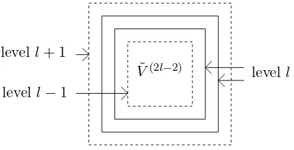
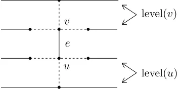
Let us first introduce some notation: Recall the definition ˜V(l) = [−l, l]2∩Z2. For l∈ N0, we say that a vertex ℓ ∈ Z2 is on level l and we write l = level(ℓ), if ℓ ∈ V˜(2l)\V˜(2(l−1)), where
we use the convention ˜V(−2) =∅. IdentifyingV(N) with the subset ˜V(N)⊂Z2, the level of ℓis also defined for vertices ℓ∈V(N). Note that the level sets are defined to have width 2 instead of width 1, see Figure 4.
Figure 4: Vertices at level lare located on the solid lines
levell−1
levell
levell+ 1
˜
V(2l−2)
Assumption 5.1 (Choice of parameters). In the following, we assume that
(i) a >0,
(ii) na= max{⌈1/√a⌉,2}, (iii) N ∈Nwith N >6na, and
In the following two definitions, we introduce a modified, truncated version of the Green’s function in 2 dimensions. At first, we take the logarithm, appropriately scaled and truncated: Definition 5.2 (Auxiliary function 1: truncated and scaled logarithm). Define a function ϕ=
ϕl,a:N0 →[0,1]by
ϕ(n) =
0 for 0≤n < na,
log(n/na) log((l−1)/na)
for na ≤n≤l−1,
1 for n≥l.
(5.1)
LetC(n):={(−n,−n),(−n, n),(n,−n),(n, n)} denote the set of corner points of the box ˜V(n). Definition 5.3(Auxiliary function 2: modified Green’s function). For everye={u, v} ∈E(N), we define a map De =D(e,N0,ℓ,a) : Ω(N) → [0,1] as follows: Let x∈ Ω(N) and l= level(ℓ). Using thisl, take ϕ=ϕl,a from Definition 5.2.
• If for some n∈N0 we have level(u) = level(v) =nor {u, v} ∩C(2n)6=∅, then we set
De(x) =ϕ(n). (5.2)
• Otherwise, we set
De(x) =
ϕ(level(u)) ifxu< xv,
ϕ(level(v)) ifxv < xu,
1
2{ϕ(level(u)) +ϕ(level(v))} ifxu=xv.
(5.3)
Thuse7→De(x) is an approximation to the Green’s function in 2 dimensions, slightly dependent on x for technical reasons. It has the property that for any vertex v not being a corner point, there is at most one edge e ∋ v with De(x) 6= ϕ(level(v)). This property is very convenient below, and it is our reason to define the level sets having width 2 instead of width 1.
We write the set E(N) of edges as a disjoint unionE(N) =F∪F′,F∩F′ =∅, whereF denotes the set of all edges e={u, v} ∈E(N) whereu and v are on the same level, and F′ denotes the set of all edges e= {u, v} ∈ E(N) with u and v on different levels. For e, e′ ∈ E(N), we write e≺e′ if and only ife∈F and e′ ∈F′. Let
Fe(N):=σ(xe′ :e′≺e) (5.4)
denote the σ-field on Ω(N) generated by the canonical projections on the coordinatese′ ∈E(N)
withe′≺e.
Lemma 5.4. For any e∈E(N), the map D
e isFe(N)-measurable.
Proof. Let e={u, v}. If level(u) = level(v) or {u, v} ∩C(2n) 6=∅ for some n∈ N0, then De is constant and there is nothing to show. By definition, our levels have thickness 2. Therefore, if
Figure 5: All vertices drawn are on leveln.
vertex in C(2n+1)
vertex in C(2n+2)
Assume that u and v are on different levels and {u, v} ∩C(n) = ∅ for all n∈ N
0. Then, De is constant on the sets {xu < xv},{xv < xu}, and {xu=xv}. Observe that
xu< xv if and only if X
e′∋u
e′6=e
xe′ <
X
e′∋v
e′6=e
xe′. (5.5)
Since u and v are on different levels, but not corner points of any box ˜V(n), all edges e′ 6= e
incident tou have endpoints on the same level, namely on level(u), see Figure 6.
Figure 6: The edgee has endpointsu and v on different levels. The edges e′ 6=e withe′ ∋u or
e′ ∋v are drawn with dashed lines.
e
u v
level(u) level(v)
Similarly, all edgese′6=eincident tov have endpoints on level(v). In other words, e′ ≺eholds for these edges e′. Thus all xe′ appearing in the two sums on the right hand side of (5.5) are
Fe(N)-measurable; recall the definition (5.4) of Fe(N). Consequently, because of (5.5), we have {xu < xv} ∈ Fe(N). The same argument shows that {xv < xu} ∈ Fe(N) and {xu = xv} ∈ Fe(N).
With these preparations, we can now introduce the deformation map Ξγ. Roughly speaking, on a logarithmic scale, the random environment xe is just shifted by γ times the approximate Green’s functionDe:
Definition 5.5 (Deformation). For any γ ∈R, we define the deformation map Ξγ = Ξ(γ,N0),ℓ,a : Ω(N)→Ω(N) by
In the following, we denote the composition of the map Ξγ : Ω(N) → Ω(N) with the map
xv : Ω(N) →(0,∞), (xe)e∈E(N) 7→
P
e∋vxe for anyv∈V(N) by
xv◦Ξγ: Ω(N)→(0,∞),(xv◦Ξγ)((xe)e∈E(N)) =
X
e∋v
exp (γDe(x))·xe. (5.7)
The following lemma collects some basic facts about this deformation map Ξγ.
Lemma 5.6 (Basic facts of the deformation map). With parameters as in Assumption 5.1, for allγ ∈R, the map Ξγ is measurable and measurably invertible. Furthermore, it has the following properties:
1. One has
x0◦Ξγ=x0 and xℓ◦Ξγ=eγxℓ. (5.8) 2. The reference measure ρ is invariant with respect toΞγ.
Proof. Letγ ∈R. The measurability of Ξγ follows from its definition (5.6) and Lemma 5.4. 1. Let x ∈ Ω(N), and let e ∈ E(N) with 0 ∈ e. Then, e∩C(0) 6= ∅, and consequently,
De(x) =ϕ(0) = 0. Hence,xe◦Ξγ=xe, and it follows thatx0 =Pe′∋0xe′ =x0◦Ξγ.
Lete∈E(N) withℓ∈e. Then,De(x) takes a value in the set{ϕ(l),ϕ(l±1), (ϕ(l) +ϕ(l± 1))/2} ={1}. Hence,xℓ◦Ξγ =eγxℓ. This completes the proof of (5.8).
2. We list the edges in E(N) in such a way that every e = {u, v} ∈ E(N) with level(u) =
level(v) gets a smaller index than every e′ = {u′, v′} ∈ E(N) with level(u′) 6= level(v′). Thus, we get a list e0, e1, . . . , eK with the property that e has a smaller index than e′ whenevere≺e′. We rewrite the definitions (5.6) of Ξ
γ and (4.2) of the reference measure
ρ in logarithmic form:
log (xe◦Ξγ) = logxe+γDe(x), (5.9)
ρ(dx) =δ1(dxe0)
Y
e∈E(N)\{e0}
dlogxe. (5.10)
SinceDeisFe(N)-measurable, we see that logxej is just translated by a value which depends
only on the componentsxei withi < j. Since 0∈e0, we haveDe0 = 0, and the component
xe0 remains unchanged. Such translations leave the reference measure ρ invariant. Here
we use that every measurable map f :Rd→Rd of the form
f(x1, . . . , xd) = (xi+gi(xj;j < i))i=1,...,d (5.11) leaves the Lebesgue measure invariant.
One verifies that the inverse of Ξγ is given by
xe◦[Ξγ]−1= exp©−γDe¡[Ξγ]−1(x)¢ªxe, (5.12)
5.2 A quadratic entropy bound
The goal of this subsection is to prove the following lemma:
Lemma 5.7 (Quadratic entropy bound). With parameters as in Assumption 5.1, for all γ ∈R
and all η∈[0,1], the image measure
Πγ,η = Π(γ,η,N)0,ℓ,a:= Ξ(γ,N0),ℓ,aP(η,N0),ℓ,a (5.13)
of Pη with respect to Ξγ is absolutely continuous with respect to Pη. If furthermore
|γ| ≤nalog
l−1
na
(5.14)
holds, one has the entropy bound
EΠγ,η
·
logdΠγ,η
dPη
¸
≤ c5(a, η)γ
2
nalog((l−1)/na)
(5.15)
with the constant
c5(a, η) := 32
µ
2a+ 1 2
¶ µ
ec6(a, η)na+ 1 log 2
>16 and (5.16)
c6(a, η) :=
½
min{√a,1} if η= 1,
1 otherwise. (5.17)
In the special caseη= 1, one has lima→0c5(a,1)<∞.
Throughout this subsection, we assume thata,na,N,ℓ, andlare fixed according to Assumption 5.1.
Forγ ∈Rand η∈[0,1], we denote by
Πγ,η− = Π(γ,η,N)−0,ℓ,a:= [Ξ(γ,N0),ℓ,a]−1P(η,N0),ℓ,a (5.18)
the image measure ofPη under the inverse of Ξγ. In the following, we suppress the dependence of De on the environmentx. Thus, we writeDe instead ofDe(x). We abbreviate forv∈V(N),
γ ∈R,T ∈ T(N), and x∈Ω(N):
xv,γ:= X
e∋v ¡
eγDex
e ¢
and YT,γ=YT,γ(x) := Y
e∈T ¡
eγDex
e ¢
. (5.19)
In order to estimate the entropy in formula (5.15), we use the following lemma. It provides an explicit formula for the logarithm of the relevant Radon-Nikodym derivative.
Lemma 5.8. 1. For anyγ ∈R and η∈[0,1], we have
Πγ,η ≪Pη ≪Π−γ,η, (5.20)
2. For any γ ∈ R and η ∈ [0,1], the Radon-Nikodym derivatives are bounded functions on
3. The following two entropies are finite and coincide:
EΠγ,η strictly positive Radon-Nikodym-derivativedPη/dρ. The reference measureρ is invariant under Ξγ by Lemma 5.6 (b). Consequently, we find
Taking ratios, this implies claim (a).
The first equality in (5.21) follows from (5.23). To prove the second equality in part (b), recall the explicit form ofdPη/dρin formula (4.10). By (5.8), we know thatx0◦Ξγ=x0andxℓ◦Ξγ=eγxℓ. Consequently, for anyγ ∈R, we obtain using (5.23) and (4.10),
dΠ−γ,η
Combining (4.10) and (5.24) yields the second equality in the claim (5.21).
Recall the definitions (5.19). Fixx∈Ω(N)and takev∈V(N)andγ ∈R. We define a probability measure µv,γ =µ(v,x,γN) on the setEv(N):={e∈E(N) :e∋v}by
µv,γ:= X
e∈E(vN)
eγDex
e
xv,γ
δe. (5.27)
For our fixed x ∈ Ω(N), we view D
• : Ev(N) → R, e 7→ De, as a random variable on the probability space (Ev(N),P(Ev(N)), µv,γ), again suppressing the dependence on the parameter x in the notation; hereP(A) denotes the power set of the setA.
Recall that we want to derive a bound for an entropy proportional to γ2. This is done by a second order Taylor expansion with respect toγ. The relevant second derivative is estimated in the following lemma.
Lemma 5.9. For all η ∈ [0,1], the function R ∋ γ 7→ log(dPη/dΠ−
γ,η) is twice continuously differentiable. The second derivative satisfies the bound
∂2 ∂2γ
·
log dPη
dΠ−γ,η ¸
≤ µ
2a+1 2
X
v∈V(N)\{0,ℓ}
Varµv,γ(D•). (5.28)
Proof. Fixx∈Ω(N). We define a probability measureν
γ=νx,γ(N) on the setT(N) by
νγ:= X
T∈T(N)
YT,γ P
T′∈T(N)YT′,γδT. (5.29)
Note that
∂
∂γxv,γ =
X
e∋v
DeeγDexe, (5.30)
∂
∂γYT,γ =
X
e∈T
DeYT,γ = ∆TYT,γ, (5.31)
where we set
∆T = ∆T(x) := X
e∈T
De. (5.32)
calculate the first and second derivative ofγ 7→log(dPη/dΠ−γ,η) using the representation (5.21):
We also calculate the second derivative:
∂2
The second order Taylor expansion for the entropy is derived in the following lemma. Lemma 5.10. The function
is twice continuously differentiable. The derivatives can be obtained by differentiating inside of the expectation, i.e. are valid for all x ∈ Ω(N). Consequently, it follows from (5.33) and (5.34) that there exists a
We know f ≥0 because entropies are always non-negative. Furthermore, since Π−0,η =Pη, we
note that the last integral is finite by (5.38).
We need another technical ingredient for the proof of Lemma 5.7. Fore={u, v} ∈E, we define because Q(ℓ,aN) is a probability measure. Hence, Proposition 4.6 of [DR06], specialized to the present model and rewritten in our present notation, claims the following equality:
EQ(N)
Intuitively, equation (5.42) has the following interpretation: We view L2e as the probability that the Markovian random walk in the environmentx traverses the edgeetwice (forward and backward) as soon as the random walker visits one of the two vertices of e. The left hand side of the equation in (5.42) is then the probability of the same event with respect to the mixture of Markov chains. On the other hand, the right hand side in the same equation equals the probability of the same event with respect to the reinforced random walk.
We have now all tools to prove the quadratic entropy bound.
Proof of Lemma 5.7. Recall Assumption 5.1. By Lemma 5.8(a), Πγ,η is absolutely continuous with respect to Pη. To prove the entropy bound (5.15), we combine first Lemma 5.8(c) with (5.37), and then we insert the bound (5.28). This yields:
Letv∈V(N)\ {0, ℓ}, and abbreviate
lv := level(v). (5.44)
Recall that the measureµv,γ =µv,x,γ(N) depends on the environment x ∈Ω(N). In the following, we stress this dependence by writingµ(v,x,γN) instead of µv,γ. To estimate the variance ofD• with
respect to the measure µ(v,x,γN) , we distinguish three cases.
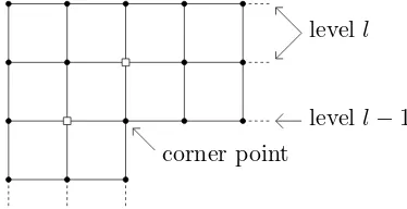
Case 1: Assume that v ∈V(N)\ {0, ℓ} is a corner point of a box [−m, m]2, i.e. v ∈C(m), for
somem≥1.
Then, there are two possibilities (see Figure 4): If m is odd, all edges incident tov have both endpoints on level lv. Otherwise, m is even and m = 2lv. In both cases, by Definition 5.3, it follows thatDe′ =ϕ(lv) for any e′ incident tov. Hence, we have the estimate:
Varµ(N)
v,x,γ(D•)≤Eµ(v,x,γN)
h
(D•−ϕ(lv))2 i
= 0. (5.45)
Case 2: Assume thatv∈V(N)\ {0, ℓ} is a neighbor of a corner pointuwith level(u)6=lv (see Figure 7).
Figure 7: The vertices marked with a square are the neighbors of corner points considered in case 2.
corner point
levell
levell−1
Then, three edges incident tov have both endpoints on levellv and one edge has one endpoint on the level of the corner point u, namely on level lv−1. Hence, for any e′ incident to v, we have De′ ∈ {ϕ(lv), ϕ(lv−1)}, and consequently
Var
µ(v,x,γN) (D•)≤Eµ(v,x,γN)
h
(D•−ϕ(lv))2 i
≤(ϕ(lv−1)−ϕ(lv))2. (5.46)
LetI denote the set of all vertices v∈V(N)\ {0, ℓ} considered in case 2. Then,
X
v∈I Var
µ(v,x,γN) (D•)≤8
∞ X
n=1
(ϕ(n+ 1)−ϕ(n))2. (5.47)
The factor 8 arises since there are 8 edges connecting corner points at levelnto vertices at level
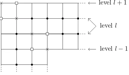
Figure 8: Corner points are marked with a cross, neighbors of corner points at a different level (as treated in case 2) are marked with a square. The black dots are the vertices at levellcovered in case 3.
levell
levell−1 levell+ 1
Then, there is precisely one vertexuadjacent tovwithlu := level(u)=6 lv. We sete(v) :={u, v}. One has De′ =ϕ(lv) for all edgese′∋v withe′6=e(v), and thus, it follows:
Var
µ(v,x,γN) (D•)≤Eµ(v,x,γN)
h
(D•−ϕ(lv))2 i
=¡
De(v)−ϕ(lv) ¢2
µ(v,x,γN) (e(v)). (5.48)
Furthermore, since we have excluded v to be as in case 2, the definition (5.3) applies to De(v).
In particular, ifxv < xu, thenDe(v) =ϕ(lv), and hence
Var
µ(v,x,γN) (D•) = 0 ifxv < xu. (5.49)
For e′ incident to v, we know that the difference De(v) −De′ takes one of the three values 0,
ϕ(lu)−ϕ(lv), and (ϕ(lu)−ϕ(lv))/2. Consequently,
µ(v,x,γN) ({e(v)}) =e γDe(v)x
e(v) xv,γ
= P xe(v)
e′∋veγ(De′−De(v))xe′
≤exp{|γ| · |ϕ(lu)−ϕ(lv)|}
xe(v) xv
. (5.50)
Assume thatxu ≤xv. Then, combining (5.48) and (5.50) and using√xuxv ≤xv yields
Var
µ(v,x,γN) (D•)≤(ϕ(lu)−ϕ(lv))
2exp
{|γ| · |ϕ(lu)−ϕ(lv)|}
xe(v)
√x uxv
. (5.51)
Because of (5.49), this estimate is also true in the case xv < xu.
A side remark: At this point, it becomes clear why in Definition 5.3,Dewas introduced in such a tricky,x-dependent way: If we had used a more naive definition ofDe instead, formula (5.51) would have failed to hold.
Integrating both sides of (5.51) with respect toPη and applying Lemma 5.11 gives
EPη
h
Var
µ(v,x,γN) (D•)
i
We sum the preceding inequality over the different verticesv:
The factor 8(4n+ 1) arises, since there are not more than 4(4n+ 1) edges connecting levelnto leveln+ 1. Each of these edges is counted at most twice, once for each of its two endpoints. By definition (5.1) ofϕ, we have
Assume thatγ satisfies (5.14):
|γ| ≤nalog
bound (5.57) in (5.53) and using (5.45), (5.47), (5.54), and (5.55) yields:
Combining this bound with (5.43) yields
The following theorem is the key to all bounds in the main theorems. One might view it as a bound for the Legendre transform of the logarithm of the partition sum EQ0[exp(ηΣℓ)]. Given
the basic facts on the deformation map Ξγ and the entropy bound from the previous section, its proof boils down to non-negativity of relative entropies.
Recall the definition (4.7) of Σℓ. We abbreviate
Q0 :=Q(0N,a). (6.1)
Hypothesis (5.14) of Lemma 5.7 is satisfied for this choice, since we have c5(a, η) > 16 for all
η∈[0,1] anda >0. Using the entropy bound (5.15) from this lemma and positivity of entropies, we get
here we used the definition (5.13) of the measure Πγ,η in the last step. Note that all expectations occurring in (6.4) are finite. As a consequence of the two equations (5.8), we find
Σℓ◦Ξγ= Σℓ+
γ
Thus, using (4.9), we find
Consequently, it follows from (6.4):
−ηγ
4 ≥logEQ0[exp(ηΣℓ)]−ηEPη[Σℓ]−
ηγ
2 . (6.7)
Combining this with our choice (6.3) forγ, we obtain the claim (6.2).
7
Tail estimates for the random environment
The following tail estimates are proved in [MR07c]. We need them for tightness arguments when we take the infinite-volume limit in Subsection 8.2, below. Recall that the random environment
clearly, the upper bound is uniform inv,w, and N. This completes the proof of (2.19).
8
Proofs of the main theorems
8.1 Uniform bounds in finite volume
Roughly speaking, Theorems 2.7 and 2.8 are just the special casesη= 1 andη= 1/2 of Theorem 6.1: l := level(v). We distinguish two cases; first finitely many exceptional cases, and then the general case.
Case 1: N ≤ 6na or l ≤ 3na. In this case, there is a path 0 = v0, v1, . . . , vk = v in V(N) joining the vertices 0 and v of length k ≤12na; recall that levels have width two. Taking the expectationEQ(N) conditions. Using reflection symmetry, we interchange 0 and v to obtain the claim (2.16):
Proof of Theorem 2.8. Leta >0,naas above, and set
Using reflection symmetry again, we interchange 0 andv in the following computation:
EP1/2[Σv] =
8.2 Bounds in infinite volume
In this subsection, we deduce the infinite-volume results Theorems 2.3, 2.4, and Theorem 2.5 from their finite volume analogs, namely Theorems 2.7, 2.8, and Lemma 2.9. First, we use a tightness argument given in the appendix to pass to the infinite volume limit.
Proof of Theorems 2.3, 2.4, and Theorem 2.5. Leta >0, and letv∈Z2. By Lemma 9.2 in the appendix, there is a measureQ0,a on Ω = (0,∞)E and a strictly increasing sequence (n(k))k∈N of natural numbers with the following properties:
a) For any finite subset F ⊂ E, the Q(0n,a(k))-distribution of (xe)e∈F converges weakly to the
Q0,a-distribution of (xe)e∈F.
b) The representation (2.7) of edge-reinforced random walk on Z2 as a mixture of Markov chains holds with the mixing measureQ0,a.
Recall from (4.1) that the weights are normalized such thatxe0 = 1 holdsQ
(n(k))
0,a -a.s. for a fixed reference edge e0 ∈E.
To prove Theorem 2.4, let v ∈ Z2 \ {0}. Since (xv/x0)1/4 takes only positive values and is a continuous function of the finitely many weightsxe withe∋v ore∋0, we conclude
EQ0,a
we used Theorem 2.8 in the last step. This proves Theorem 2.4. Using (2.18) from Lemma 2.9, the same argument yields Theorem 2.5.
To prove Theorem 2.3, we observe that log(xv/x0) is also a continuous function of the finitely
many weights xe with e∋v ore∋0. Let 0 =v0,v1,. . .,vL=v be a path from 0 to v, and let
Consequently, for any fixed vertex v, the law of log(xv/x0) with respect to Q(0N,a) is uniformly integrable in N for large N. Abbreviating fM(x) := (x∧M)∨(−M) for the truncation at M and −M, we get, using uniform integrability to interchange limits:
EQ0,a
The last inequality follows from the bound (2.16).
8.3 Hitting probabilities for ERRW
Finally, we apply our bounds for the random environment to deduce estimates for the hitting probabilities for the edge-reinforced random walk.
Proof of Theorem 2.1. 1. We claim first that for allx∈Ω and allv∈Z2\{0}, the probability
Q0,x[τv < τ0] for the random walk starting in 0 in the fixed environmentx to visitv before
returning to 0 and the probabilityQv,x[τ0< τv] for the random walk with exchanged roles of 0 andv in the same environment are connected by the following equation:
Q0,x[τv < τ0] = xv
x0
Qv,x[τ0< τv]. (8.16)
To prove this claim, take two vertices u 6= w. Denote by Πu,w the set of all admissible finite paths
π = (u=v0, v1, . . . , vn=w), (8.17)
n∈N, joining u and w, which visit u orw precisely once, namely at the end points. For any such pathπ, we introduce the event
Aπ :={Xi =vi fori= 0,1, . . . , n} ⊆(Z2)N0 (8.18)
that π is an initial piece of the random path. Note that the events Aπ, π ∈ Πu,w, are pairwise disjoint. Furthermore, let
π↔:= (vn, . . . , v1, v0) (8.19)
denote the reversed path. Note that the reversion defines a bijection ·↔ : Π
0,v → Πv,0.
Moreover, for any pathπ as in (8.17),
Now, we take u = 0 and w =v. Summing (8.20) over all π ∈Π0,v, we obtain the claim (8.16) as follows:
x0Q0,x[τv < τ0] =x0
X
π∈Π0,v
Q0,x[Aπ] =xv X
π∈Π0,v
Qv,x[Aπ↔]
=xv X
π∈Πv,0
Qv,x[Aπ] =xvQv,x[τ0< τv]. (8.21)
From this, we conclude
Q0,x[τv < τ0]≤ xv
x0
. (8.22)
Taking the 1/4-th power and expectations yields
P0,a[τv< τ0] =EQ0,a[Q0,x[τv< τ0]]≤EQ0,a[Q0,x[τv < τ0]
1/4]
≤EQ0,a
" µ
xv
x0
¶1/4#
≤c1(a)|v|−β(a); (8.23)
we used the representation of the edge-reinforced random walk as a random walk in random environment from Theorem 2.2 in the first step and the bound (2.10) from Theorem 2.4 in the last step. This shows part (a) of Theorem 2.1.
2. To prove part (b), let Σnu,w denote the set of all admissible paths
π= (u=v0, v1, . . . , vn=w) (8.24)
from u to w of lengthn. Again, reversion yields a bijection between Σnu,w and Σnw,u, and the events Aπ,π ∈Σnu,w, are pairwise disjoint. In analogy to (8.21), we obtain
x0Q0,x[Xn=v] =x0
X
π∈Σn
0,v
Q0,x[Aπ] =xv X
π∈Σn v,0
Qv,x[Aπ] =xvQv,x[Xn= 0]. (8.25)
Using this, an analogous argument to (8.23) yields the claim (2.2).
9
Appendix
9.1 Proof of Lemma 4.1
In this appendix, we consider a generalization of Lemma 4.1 to arbitrary finite graphs. It essentially states the formula of Coppersmith and Diaconis [CD86] for the law of the random environment, transformed to a special normalization.
Consider edge-reinforced random walk on any finite graph (V, E) with starting pointv0 ∈V and
initial weights a= (ae)e∈E ∈(0,∞)E. Recall definition (2.8) ofxv; we use the similar notation
av=Pe∋vae. Forx= (xe)e∈E ∈(0,∞)E, we set
φv0,a(x) =c10(v0, a)
Q
e∈Exaee−1
xav0/2
v0
Q
v∈V\{v0}x
(av+1)/2
v
s X
T∈T Y
e∈T
where the sum is indexed by the set T of all spanning trees of (V, E), viewed as sets of edges,
Lemma 9.1. The above edge-reinforced random walk on (V, E) has the same distribution as a random walk in a random environment given by random positive weights x˜ = (˜xe)e∈E on
Note that the normalizing constant c10(v0, a) does not depend on the choice of the reference
edgee0.
Proof. By Theorem 3.1 of [Rol03], the edge-reinforced random walk on (V, E) has the same distribution as a random walk in a random environment given by random positive weights
x = (xe)e∈E on the edges. The law of the random environment Q∆v0,a, normalized such that
P
e∈Exe = 1, has a density with respect to the normalized surface measure on the simplex ∆ = {(xe)e∈E ∈ (0,∞)E | Pe∈Exe = 1}. The density is provided by Theorem 1 in [KR00]. Combining this theorem with the matrix-tree-theorem ([Mau76], p. 145, Theorem 3’, see also Theorem 3 in [KR00]), it is given by
dQ∆v
0,a
dσ (x) =
φv0,a(x)
(|E| −1)!. (9.3)
Consider the change of normalization
F : ∆→H, F((xe)e∈E) =
where the first map is the canonical projection and the last map ι just includes an extra com-ponent ˜xe0 = 1. Let us calculate the Jacobi determinant of the mapf. Using the abbreviation
xe0 = 1−
holds for rank 1 matrices A, we get the Jacobi determinant
Abbreviating
α:=X
e∈E
ae− |E| − X
v∈V
av 2 −
|V| −1
2 =−|E| −
|V| −1
2 =−|E| −
|T|
2 (9.8)
for any spanning tree T ⊆E in (V, E), we rewrite (9.1) as
φv0,a(x) =c10(v0, a)x
α e0
Q
e∈Ex˜aee−1 ˜
xav0/2
v0
Q
v∈V\{v0}x˜
(av+1)/2
v
s X
T∈T
x|eT0|
Y
e∈T ˜
xe=xe−|0E|φv0,a(˜x) (9.9)
and thus
φv0,a(x)
detDf(π(x)) =φv0,a(˜x). (9.10)
We combine this with (9.3). Using that the projected normalized surface measure πσ has the density (|E| −1)! with respect to the Lebesgue measure on π[∆], we get that the transformed distribution Qv0,a = FQ∆v0,a has the density φv0,a(˜x) with respect to the Lebesgue measure
δ1(dx˜e0)
Q
e6=e0dx˜e on the hyperplaneH. This proves the claim.
9.2 A tightness argument for infinite-volume limits
In this appendix, we prove a variant of Lemma 5.3 of [MR07c] for more general graphs. Con-sider any infinite, locally finite, undirected, weighted graph G∞ = (V∞, E∞, a) with vertex
set V∞, edge set E∞ and positive weights a = (ae)e∈E∞ on the edges. Furthermore, let
GN = (VN, EN, aN),N ∈N, be a sequence of finite, undirected, weighted graphs with weights
aN = (aN,e)e∈EN ∈(0,∞)
EN. Finally, let ˜G
N = ( ˜VN,E˜N,˜aN),N ∈N, be an increasing sequence of connected weighted subgraphs ofG∞ with the weights ˜aN induced byG∞ with the following
properties:
1. For anyN, ˜GN is a full subgraph ofG∞, i.e., for every edgee∈E∞withe⊆V˜N, one has
e∈E˜N.
2. One has ˜VN ↑V∞ asN → ∞.
3. Furthermore, for anyN, the graph ˜GN is also a full weighted subgraph ofGN. In particular, restricted to ˜EN, the weights onGN and on G∞ coincide.
Take a starting point 0 ∈ V˜0 and a reference edge e0 ∈ E˜0. Consider edge-reinforced random
walk on GN and on G∞ with starting point 0 and initial weightsaN and a, respectively. Let
QN denote the distribution of the random environment on (0,∞)EN in the representation of
the edge-reinforced random walk onGN as in Lemma 9.1, normalized such that xe0 = 1 holds
QN-almost surely. The following lemma is a variant of Lemma 5.3 in [MR07c]. In that paper, we consider the special case ˜GN =GN. Boxes with periodic boundary conditions, as needed in our application, are not covered by the cited lemma.
Lemma 9.2. There exist a probability measure Q∞ on (0,∞)E∞ and a strictly increasing
(a) For any finite subset F ⊂E∞, the Qn(k)-distribution of (xe)e∈F converges weakly to the
Q∞-distribution of (xe)e∈F as k→ ∞.
(b) Edge-reinforced random walk on G∞, started in 0, has the same law as a random walk in
a random environment, where the random environment is distributed according to Q∞.
Proof. We construct Q∞ by a tightness and diagonalization argument. We claim: For every
e∈E∞ and every N0 ∈N with e∈ E˜N0, the sequence of laws ([logxe]QN)N≥N0 of logxe with
respect toQN is tight. To see this, fix a path of edges e0, e1, . . . , ek starting in e0 and ending in e=ek. Now, Theorem 2.4 in [MR07c] claims that for allM >0
QN[xe≥M xe0]≤c11M
−c12 and Q
N[xe0 ≥M xe]≤c11M
−c12 (9.11)
holds with some positive constants c11 and c12, depending on the initial weights aand on the
pathe0, e1, . . . , ek, but notdepending onN. Sincexe0 = 1 holds QN-almost surely, this implies
the tightness claimed above. We recursively construct a sequence of strictly increasing sequences (nk,N)k∈N,N ∈Nwithnk,N ≥N for allk and N, with the following properties:
(i) (nk,N+1)k∈Nis a subsequence of (nk,N)k∈N for allN.
(ii) The joint law of (logxe)e∈E˜N with respect to Qnk,N converges weakly ask→ ∞ for allN.
For N = 0, using tightness, there exists a strictly increasing sequences (nk,0)k∈N of natural numbers such that (ii) holds for N = 0. For the recursion step N ❀ N + 1, using tightness again, choose a subsequence (nk,N+1)k∈Nof (nk,N)k∈Nsuch that (ii) holds also forN+1. Finally, take the diagonal sequencen(k) :=nk,k. Then, for allN ∈N, the law of (xe)e∈E˜N with respect
to Qn(k) converges weakly as k → ∞ to some distribution ˜QN on (0,∞)E˜N. By construction,
the projection of ˜QN+1 to (0,∞)E˜N coincides with ˜Q
N. Thus Kolmogorov’s extension theorem yields a probability measureQ∞on (0,∞)E∞ with marginals ˜Q
N for allN; recall that ˜EN ↑E∞
asN → ∞. By construction, claim (a) of the lemma is true.
The proof of part (b) is very similar to the proof of the first part of Lemma 5.1 in [MR06a]. For completeness, we repeat the argument. We claim that the law P0,a of the edge-reinforced law on G∞ has the following representation:
P0,a[A] = Z
(0,∞)E∞
Q0,x[A]Q∞(dx) (9.12)
for all events A of admissible paths, where Q0,x denotes the law of a Markovian random walk on G∞ in the fixed environment x. Events of the form A = {(Xs)s=0,...,m−1 = π}, (π ∈ Vm
an admissible path, m∈N), together with the empty set, generate the canonical σ-field on the space of admissible paths and form a closed system with respect to intersection. Thus it suffices to check (9.12) for these events. Fix m ∈ N and π ∈Vm
∞. Without loss of generality we may
assume thatπ is a path inG∞ starting in 0. LetN ∈Nbe so large thatπ and all edges in E∞
˜
GN, andGN. Using the representation of the edge-reinforced random walk onGN as a mixture of Markov chains Q0,x with mixing measureQN(dx) (Lemma 9.1), this implies
P0,a[(Xs)s=0,...,m−1 =π] =
Z
(0,∞)EN Q0,x[(Xs)s=0,...,m−1=π]
QN(dx) (9.13)
for sufficiently large N. Taking the limit along the sequence (n(k))k∈N yields the claim (9.12) as follows:
P[(Xs)s=0,...,m−1 =π] = lim
k→∞ Z
(0,∞)En(k)
Q0,x[(Xs)s=0,...,m−1 =π]Qn(k)(dx)
=
Z
(0,∞)E∞
Q0,x[(Xs)s=0,...,m−1 =π]Q∞(dx). (9.14)
Acknowledgement: The authors would like to thank two anonymous referees for carefully reading the paper.
References
[CD86] D. Coppersmith and P. Diaconis. Random walk with reinforcement. Unpublished manuscript, 1986.
[DF80] P. Diaconis and D. Freedman. de Finetti’s theorem for Markov chains. Ann. Probab., 8(1):115–130, 1980. MR0556418
[Dia88] P. Diaconis. Recent progress on de Finetti’s notions of exchangeability. In Bayesian statistics, 3 (Valencia, 1987), pages 111–125. Oxford Univ. Press, New York, 1988. MR1008047
[DR06] Persi Diaconis and Silke W. W. Rolles. Bayesian analysis for reversible Markov chains. Ann. Statist., 34(3):1270–1292, 2006. MR2278358
[KR00] M.S. Keane and S.W.W. Rolles. Edge-reinforced random walk on finite graphs. In Infinite dimensional stochastic analysis (Amsterdam, 1999), pages 217–234. R. Neth. Acad. Arts Sci., Amsterdam, 2000. MR1832379
[Mau76] S. B. Maurer. Matrix generalizations of some theorems on trees, cycles and cocycles in graphs. SIAM Journal on Applied Mathematics, 30(1):143–148, 1976. MR0392635 [MR05] F. Merkl and S.W.W. Rolles. Edge-reinforced random walk on a ladder. Ann. Probab.,
33(6):2051–2093, 2005. MR2184091
[MR06b] F. Merkl and S.W.W. Rolles. Linearly edge-reinforced random walks. In D. Denteneer, F. den Hollander, and E. Verbitskiy, editors,Dynamics and Stochastics: Festschrift in Honor of M.S. Keane, volume 48 of IMS Lecture Notes Monogr. Ser., pages 66–77, 2006. MR2306189
[MR07a] F. Merkl and S.W.W. Rolles. Asymptotic behavior of edge-reinforced random walks. The Annals of Probability, 35(1):115–140, 2007. MR2303945
[MR07b] F. Merkl and S.W.W. Rolles. Recurrence of edge-reinforced random walk on a two-dimensional graph. Preprint available from http://arxiv.org/abs/math.PR/0703027, 2007.
[MR07c] Franz Merkl and Silke W. W. Rolles. A random environment for linearly edge-reinforced random walks on infinite graphs. Probab. Theory Related Fields, 138(1-2):157–176, 2007. MR2288067
[Pem88] R. Pemantle. Phase transition in reinforced random walk and RWRE on trees. Ann. Probab., 16(3):1229–1241, 1988. MR0942765
[Rol03] S.W.W. Rolles. How edge-reinforced random walk arises naturally. Probab. Theory Related Fields, 126(2):243–260, 2003. MR1990056
[Rol06] S.W.W. Rolles. On the recurrence of edge-reinforced random walk on Z×G. Probab. Theory Related Fields, 135(2):216–264, 2006. MR2218872