O R I G I N A L R E S E A R C H
Open Access
A multi-objective model for designing a group
layout of a dynamic cellular manufacturing
system
Reza Kia
1*, Hossein Shirazi
2, Nikbakhsh Javadian
3and Reza Tavakkoli-Moghaddam
4Abstract
This paper presents a multi-objective mixed-integer nonlinear programming model to design a group layout of a cellular manufacturing system in a dynamic environment, in which the number of cells to be formed is variable. Cell formation (CF) and group layout (GL) are concurrently made in a dynamic environment by the integrated model, which incorporates with an extensive coverage of important manufacturing features used in the design of CMSs. Additionally, there are some features that make the presented model different from the previous studies. These features include the following: (1) the variable number of cells, (2) the integrated CF and GL decisions in a dynamic environment by a multi-objective mathematical model, and (3) two conflicting objectives that minimize the total costs (i.e., costs of intra and inter-cell material handling, machine relocation, purchasing new machines, machine overhead, machine processing, and forming cells) and minimize the imbalance of workload among cells. Furthermore, the presented model considers some limitations, such as machine capability, machine capacity, part demands satisfaction, cell size, material flow conservation, and location assignment. Four numerical examples are solved by the GAMS software to illustrate the promising results obtained by the incorporated features.
Keywords:Dynamic cellular manufacturing systems, Multi-objective model, Cell formation, Group layout
Introduction
Cellular manufacturing (CM), which is an innovative manufacturing strategy derived from a group technology concept, can be employed in order to improve both the flexibility and efficiency in today's modern competitive manufacturing environments (e.g., flexible manufacturing systems and just-in-time production). The design steps of a cellular manufacturing system (CMS) include the follow-ing: (1) cell formation (CF) (i.e., clustering parts with simi-lar processing requirements into part families and related machines into machine cells), (2) group layout (GL) (i.e., intra-cell layout arranging machines within each cell, and inter-cell layout arranging cells with regard to each other), and (3) group scheduling (GS) (i.e., scheduling part fam-ilies) (Wemmerlov and Hyer 1986).
Unplanned changes in the product mix and demand volume necessitate reconfiguration of layouts of modern
manufacturing systems producing multiple products and working in highly unstable environments. Hence, ignor-ing these changes such as new products in the comignor-ing future imposes subsequent unplanned changes to the CMS and causes production disruptions and unexpected costs. As a result, product life cycle changes should be incorporated in the design of cells. This type of the sys-tem is called the dynamic cellular manufacturing syssys-tem (DCMS) (Rheault et al. 1995). Drolet et al. (2008) devel-oped a stochastic simulation model and indicated that DCMSs are generally more efficient than classical CMSs or job shop systems, especially with respect to performance measures (e.g., the throughput time, work-in-process, tar-diness, and the total marginal cost) for a given horizon.
Reconfiguring cells incurs the corresponding costs (e.g., moving machines, installing or uninstalling machines, lost production time, and relearning). By considering the re-configuration costs, it is possible that a suboptimal config-uration is the best one to utilize in a period because utilizing this may impose lower reconfiguration and overall costs (Balakrishnan and Cheng 2007). Thus, when creating * Correspondence:[email protected]
1Department of Industrial Engineering, Firoozkooh Branch, Islamic Azad University, P.O. Box 148, Firoozkooh, Iran
Full list of author information is available at the end of the article
© 2013 Kia et al.; licensee Springer. This is an Open Access article distributed under the terms of the Creative Commons Attribution License (http://creativecommons.org/licenses/by/2.0), which permits unrestricted use, distribution, and reproduction in any medium, provided the original work is properly cited.
manufacturing cells, it is important to consider the recon-figuration cost of cells.
Since our model integrates CF and GL decisions in a dynamic environment, we actually incorporate a dynamic layout problem in a DCMS model. In this case, an appro-priate decision should be made among the available strat-egies (e.g., purchasing a new machine to meet increased demand requirements, relocating the machine that is un-derutilized in a cell to another cell where demand require-ments are higher, and re-planning the part production) in order to make a trade-off between resultant costs of pur-chasing machine, reconfiguration, and intra- and inter-cell material handling.
Wemmerlov and Johnson (2000) indicated that the prac-tical implementation of a CMS involves the optimization of many conflicting objectives. For example, minimizing the total cell load variations worsens the objectives of minimiz-ing the outsourcminimiz-ing cost and inter-cell material handlminimiz-ing cost because it necessitates some of parts to be outsourced or some of the processing operations in cells to be shifted to another. A detailed description of the multi-objective optimization can be found in Collette and Siarry (2003).
The aim of this paper is to present a multi-objective mathematical model with an extensive coverage of im-portant manufacturing features consisting of alternative process routings, operation sequence, processing time, pro-duction volume of parts, purchasing machine, duplicate machines, machine capacity, lot splitting, group layout, multi-rows layout of equal area facilities, flexible reconfigur-ation of cells, variable number of cells, and balancing of the cell workload. The first objective of our presented model re-lated to cost components is to minimize the total costs of intra- and inter-cell material handling, machine relocation, purchasing new machines, machine overhead cost, machine processing, and forming of cells. The second objective is to minimize the imbalance of workload among cells.
The model presented in this study is an extended ver-sion of the integrated model proposed by Kia et al. (2012) in which the excellent advantages are (1) multi-rows lay-out of equal-sized facilities, (2) flexible configuration of cells, (3) calculating relocation cost based on the locations assigned to machines, (4) distance-based calculation of intra- and inter-cell material handling costs, (5) consider-ing intra-cell movements between two machines of a same type, (6) applying the equations of material flow conserva-tion, and (7) integrating the CF and GL decisions in a dy-namic environment.
This study also incorporates some other important as-pects in comparison with the previous study carried out by Kia et al. (2012) and the models presented in the lit-erature. In the first aspect, finding the optimal number of cells provides the flexibility for the model to form cells in optimal numbers to reduce the total costs especially be-cause of simultaneously reducing the cost of forming cells
and improving the CM utilization. In the second aspect, we consider two conflicting objectives that minimize the total costs and minimize the imbalance of workload among cells. In the third aspect, the CF and GL decisions are integrated in a dynamic environment by a multi-objective mathematical model incorporating with several design features. The importance of the incorporated fea-tures in improving the performance of the extended model is revealed by numerical examples.
The remainder of this paper is organized as follows. The literature review related to the DCMS, GL, and multi-objective cell formation problem is presented in the‘ Litera-ture review’section. In the ‘Mathematical model’section, a multi-objective mathematical model integrating DCMS and GL decisions is presented.‘Computational results’section il-lustrates the test problems that are utilized to investigate the features of the presented model. Finally, conclusion is given.
Literature review
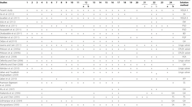
In this section, we present the related literature review of studies addressing layout problems, multi-objective mathematical modeling, and dynamic issues in designing a CMS. Since a comprehensive literature review related to layout problems and dynamic issues in designing a CMS has been done by Kia et al. (2012), here we summarize recent studies of DCMS issue in Table 1.
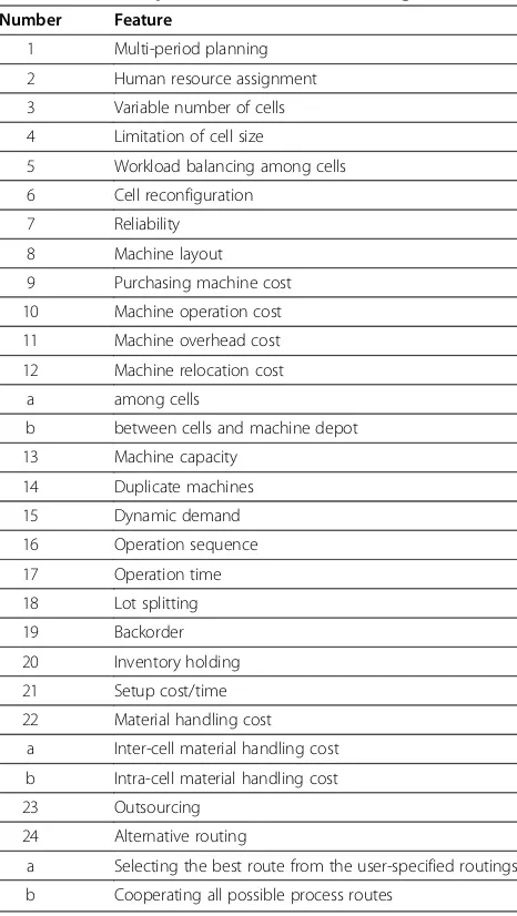
A list of important features proposed for the CM de-sign is given in Table 2. We investigate 23 recently pub-lished papers considering the majority of corresponding features as presented in Table 2. The model presented in this paper includes a larger coverage of the features than the individual papers presented in Table 1.
Mathematical model
In this section, the integrated problem is formulated under the following assumptions:
1. Each part type has a number of operations that must be processed based on its operation sequence. 2. The demand for each part type in each period is known. 3. The capabilities of part operations processing and
processing time of part operations for each machine type are known.
4. Each machine type has a limited capacity expressed in hours during each time period.
5. Machines can have one or more identical duplicates to satisfy capacity requirements.
6. The overhead cost of each machine type is known and implies maintenance and other overhead costs, such as energy cost and general service.
Table 1 Important features in the CM design used in this research and other recent studies
Studies 1 2 3 4 5 6 7 8 9 10 11 12 13 14 15 16 17 18 19 20 21 22 23 24 Solution method
a b a a b a b
Present study x x x x x x x x x x x x x x x x x x x x x x NSGA II
Kia et al. (2012) x x x x x x x x x x x x x x x x x SA
Javadian et al. (2011) x x x x x x x x x x x x x x x x x x x x NSGA II
Jolai et al. (2012) x x x x x x EM
Rafiee et al. (2011) x x x x x x x x x x x x x x x x x x PSO
Rezazadeh et al. (2011) x x x x x x x x x x x x PSO
Ghotboddini et al. (2011) x x x x x x x x x x x x x x x x x BD
Mahdavi et al. (2011) x x x x x x x x x x x FGP
Deljoo et al.(2010) x x x x x x x x x x x x x GA
Saxena and Jain (2011) x x x x x x x x x x x x x x x x x x x x Lingo solver
Ahkioon et al. (2009a) x x x x x x x x x x x x x x x x x CPLEX solver
Ahkioon et al. (2009b) x x x x x x x CPLEX solver
Safaei et al. (2008) x x x x x x x x x x x x x x HSA
Defersha and Chen (2006) x x x x x x x x x x x x x x x x x x Lingo solver
Defersha and Chen (2008) x x x x x x x x x x x x x x x x x x GA
Mahdavi et al. (2010) x x x x x x x x x x x x x x x x Lingo solver
Safaei and Tavakkoli-Moghaddam (2009)
x x x x x x x x x x x x x x
x x Lingo solver
Safaei et al. (2010) x x x x x x x x x x IFP
Aramoon Bajestani et al. (2009)
x x x x x x x x x x x x x x SS
Wu et al. (2007) x x x x x x GA
Nsakanda et al. (2006) x x x x x x x GA GA
Cao and Chen (2005) x x x x x x x x x x TS TS
Solimanpur et al. (2004) x x x x x x x x x GA GA
Mungwattana (2000) x x x x x x x x x x x x x x x SA SA
BD, Bender's decomposition; EM, electromagnetism-like method; FGP, fuzzy goal programming; GA, genetic algorithm; HSA hybrid simulated annealing; IFP interactive fuzzy programming; NSGA-II elitist non-dominated sorting genetic algorithm; PSO, particle swarm intelligence; SA, simulated annealing; SS, scatter search; TS, Tabu search.
Kia
et
al.
Journal
of
Industria
l
Engineerin
g
Internationa
l
2013,
9
:8
Page
3
of
14
http://ww
w.jiei-tsb.com
/content/9/
machines cannot satisfy the part demand, some other machines will be purchased and added to the currently utilized machines.
8. The variable cost of each machine type implying the operating cost of that machine is dependent on the workload assigned to the machine and is known. 9. Cell reconfiguration involves transferring of the
existing machines between different locations and purchasing and adding new machines to cells. 10. To reconfigure the cells, there is no need to alter the
foundations or modify the buildings. By considering this assumption, reassigning machines to cells will not impose any reconfiguration cost, unless the machines are relocated between different locations. 11. The transferring cost of each machine type between
two periods is known. This cost is paid for two situations: (1) to install a newly purchased machine and (2) to transfer a machine between two locations of
a same cell or different cells. In addition, it is assumed that the unit cost of adding or removing a machine to/ from the cells is half of the machine transferring cost. 12. Inter- and intra-cell movements related to the part
types have different costs. The material handling cost of inter- and intra-cell movements is related to the distance traveled. In other words, it is assumed that the distance between each pair of machines is dependent on locations assigned to those machines. Machines should be placed in the locations, whose distance from each other is known in advance, and therefore the distance matrix,D¼ dll0
h i
, is known wheredll0 represents the distance between locations
l andl'(l,l'= 1,…,L). All machine types have the same dimensions and are placed in the locations also with the same dimensions.
13. The maximum number of cells which can be formed in each period must be specified in advance. However, the number of cells which should be formed in each period is considered as a decision variable.
14. The maximum and minimum of the cell size are known in advance.
15. All machine types are assumed to be multi-purposed ones, which are capable to perform one or more operations without imposing a reinstalling cost. In the same manner, each operation of a part type can be performed on different machine types with different processing times.
16. A part operation can be distributed between several machines which are capable to process that operation within the same cell or even in different cells (lot splitting).
17. The number of locations is known in advance. 18. The workload of the cells should be balanced.
The following notations are used in the model:
Sets
P= {1,2,…,P} index set of part types
K(p) = {1,2,…,Kp} index set of operations indices for part typep
M= {1,2,…,M} index set of machine types
C= {1,2,…,C} index set of cells
L= {1,2,…,L} index set of locations
T= {1,2,…,T} index set of time periods
Model parameters
IEp inter-cell material handling cost per part type p per unit of distance
IAp intra-cell material handling cost per part type p per unit of distance
Dpt demand for part typepin periodt Table 2 List of important features in CM design
Number Feature
1 Multi-period planning
2 Human resource assignment
3 Variable number of cells
4 Limitation of cell size
5 Workload balancing among cells
6 Cell reconfiguration
7 Reliability
8 Machine layout
9 Purchasing machine cost
10 Machine operation cost
11 Machine overhead cost
12 Machine relocation cost
a among cells
b between cells and machine depot
13 Machine capacity
14 Duplicate machines
15 Dynamic demand
16 Operation sequence
17 Operation time
18 Lot splitting
19 Backorder
20 Inventory holding
21 Setup cost/time
22 Material handling cost
a Inter-cell material handling cost
b Intra-cell material handling cost
23 Outsourcing
24 Alternative routing
a Selecting the best route from the user-specified routings
Tm capacity of one unit of machine typem
C maximum number of cells that can be formed in each period
FCt cost of forming a cell in periodt BU upper cell size limit
BL lower cell size limit
tkpm processing time of operationkon machinemper part typep
d
ll0 distance between two locationslandl' αm overhead cost of machine typem
βm variable cost of machine typemfor each unit time akpm 1 if operation k of part p can be processed on machine typem;0, otherwise
γm purchase cost of machine typem
δm transferring cost per machine typem Decision variables
Xkpmlt number of parts of typepprocessed by operation kon machine typem'located in locationl'in periodt Wmlct 1 if one unit of machine typemis located in lo-cationland assigned to cellcin periodt;0, otherwise Y
kpmlm0l0t number of parts of typepprocessed by
oper-ationkon machine typemlocated in locationland moved to the machine typem’located in locationl’in periodt Yct 1 if cellcis formed in periodt;0, otherwise NPmt number of machine typempurchased in periodt
The DCMS mathematical model
The DCMS model is extended and formulated as multi-objective mixed-integer non-linear programming:
minZ1¼∑
The first objective function consists of seven cost com-ponents. Term (1.1) is the intra-cell material handling
Kiaet al. Journal of Industrial Engineering International2013,9:8 Page 5 of 14
cost. This cost is incurred if consecutive operations of the same part type are processed in the same cell, but on different machines. For instance, operation kof part typepis processed on machine typemassigned to loca-tion lin cell c at timet. If the next operation, k+ 1, of partp is processed on any other machine, but within the same cell, then an intra-cell cost is incurred. The product
WmlctWm0
l0ct in term (1.1) is to verify whether two
ma-chines of typesmandm′assigned to locationslandl′are in the same cell. If the product reflects 1 as the result, then those machines, which are in a same cell and the material flow between them, impose the intra-cell material handling cost. To calculate this cost, the material flow between the
machines assigned in the same cell Ykpmlm0
l0t
is
multi-plied to the distance between the locations of those
ma-chines dll0
, and then to the intra-cell material handling cost per each part type (IAp). This term of the objective function tries to locate two machines having a large quan-tity of the material flow near each other in order to shorten the distance between them and to assign those machines in the same cell to pay the intra-cell material handling cost (IAp) lesser than the inter-cell material handling cost (IEp), and finally to take a small portion in the objective function.
In a similar way, term (1.2) denotes the inter-cell ma-terial handling cost. This cost is incurred whenever con-secutive operations of the same part type are transferred between different cells. For instance, assume that oper-ation k of part type p is processed on machine type m
in cell c at time t. If the next operation (i.e., k + 1) of partpis processed on any machine, but in another cell, then an inter-cell cost is incurred. To decrease this section of the objective function, it is better to locate two machines having a small quantity of the material flow between each other in different cells rather than those machines having a large quantity of the material flow in order to pay the inter-cell material handling cost (IEp) for a smaller quantity of the material flow of parts between different cells.
Term (1.3) represents the reconfiguration cost of cells oc-curring in (1) installing a new purchased machine or (2) transferring a machine between two locations in the cells. The component ∑C
cWmlct−∑CcWmlc;tþ1
in term (1.3) quests
whether machine typemassigned to locationlin periodt
remains in the same location for subsequent period,t+ 1. The component ∑CcWmlct−∑CcWmlc;tþ1
equaling to value 1
means that an installation or uninstallation of machine type
m in locationl is happened. Thus, based on Assumption (11), a half of transferring machine cost (δm) for machine typemshould be paid. In the other hand, the component
∑C
cWmlct−∑CcWmlc;tþ1
equaling to value 2 means a
trans-ferring of machine typembetween two different locations in the cells has happened and a complete transferring ma-chine cost (δm) for machine type m should be paid. The
lates installation costs for the newly purchased machines in the first period (t= 1).
Term (1.4) is the purchase costs of new machines. Term (1.5) incorporates the overhead costs. Term (1.6) takes into account the operating costs of all machine types. Term (1.7) is the total costs of forming cells.
The second objective function pertains to the total cell load variation. Balancing workload between the cells re-duces work-in-process inventory, improves material flow through the cells, and prevents overutilization of some cells and underutilization of others (Baykasoglu et al. 2001). In this paper, the total cell load variation in each period is measured by calculating the absolute deviation between the workload of each cell and average workload of cells.
Inequality (2) guarantees that each operation of a part is processed on the machine, which is capable to process that operation. Constraint (3) shows that the demand of each part should be satisfied in a period through internal production. Equation (4) describes that the number of machine typemutilized in the periodtis equal to num-ber of utilized machines of the same type in the previous period plus the number of new machines of the same type purchased at the beginning of the current period. The cell size is limited through Constraints (5) and (6), where the cell size lies within the user defined lower and upper bounds. Constraint (7) is related to the machine capacity. Constraints (8) and (9) are material flow con-servation equations. Constraint set (10) is to ensure that each location can receive one machine at most and only belong to one cell, simultaneously. Constraints (11) to (13) provide the logical binary and non-negativity integer necessities for the decision variables.
Computational results
Illustrative numerical examples for the single-objective model
To validate the proposed model and illustrate its various features, a test problem taken from the example (Kia et al. 2012) is solved using GAMS 22.0 software (solver CPLEX) (Washington, DC, USA) on an Intel(R) Core (TM)2 Duo CPU @2.66 GHz (Intel Corporation, Santa Clara, CA, USA) with 4 GB RAM. In this section, only the objective functionZ1cost components is considered
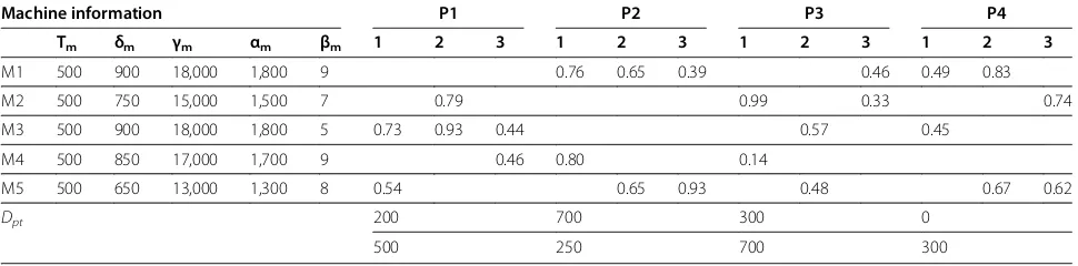
operating cost. For more simplicity, the capacity of all machines is assumed to be equal to 500 h per period. Furthermore, the processing time of each operation for all part types are presented in Table 3. In addition, the demand quantity for each part type and the product mix for each period are presented in this table. The forming cell cost, intra- and inter-cell material handling costs per each part type are 20,000; 5; and 50; respectively.
The maximum number of cells formed in each period is four. Also, the lower and upper sizes of cells are 2 and 3, respectively. The distances between eight locations existing in the shop floor are presented in the matrix, as shown in Table 4.
The obtained solution with the model presented in this paper on the explained example is detailed out. Also, to show the advantage of the proposed model and consider-ing the variable number of cells in comparison with to the previous model (Kia et al. 2012), the solutions obtained using two models and their performance are discussed in the rest of this section. The presented model consists of 652,619 variables and 751,238 constraints in the given ex-ample. The optimal solution is obtained after 74,159 s (i.e., about 20 h). This reveals the NP-hardness of the presented model even in solving such a small-sized example.
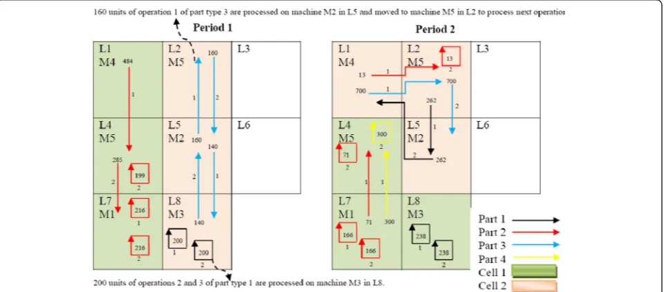
The cell configurations and machine layout for two periods corresponding to the best solutions obtained using the model (Kia et al. 2012) with three cells and the presented model with two optimal cells are shown in
Figures 1 and 2, respectively. These figures show some of the characteristics and advantages of the presented model with variable number of cells.
As can be seen, for the model with optimal number of cells, two cells in each period are formed that reduces the forming cell cost in comparison with the previous model where forming three cells had been predetermined by system designer. Also, in the first period, one quantity of machine types 1, 2, 3, and 4 and two quantities of ma-chine type 5, six mama-chines in total, are purchased. In the second period, it is not required to purchase new ma-chines and to increase the available machine capacity. In the first period, machine types 4, 5, and 1 are assigned to cell 1 and in locations 1, 4, and 7, respectively. Further-more, in the first period machine types 5, 2, and 3 are assigned to cell 2 and in locations 2, 5, and 8, respectively. In the second period, the locations of machines will be un-changed, but the configuration of cells will be changed as machine type 4 (M4) assigned to cell 1 and located in lo-cation 1 (L1) in period 1 will be assigned to cell 2 in period 2 and in a similar way machine M3 assigned to cell 2 and located in L8 in period 1 will be assigned to cell 1 in period 2. As a result, relocating machines is not necessary between two successive periods. Since there is no machine relocation between periods, the only cost which is in-curred for relocation is related to installing new purchased machines in the first period.
In addition, Figure 2 shows a further illustration of the material flows between the machines represented by di-rected arcs. For instance, in period 1 the quantity of the first operation of part 2 processed on machine 4 in loca-tion 1 of cell 1 is 484 units, from which 199 parts are processed by operations 2 and 3 on the machine 5 in lo-cation 4 of cell 1, and the remaining 285 units are processed by operation 3 on the machine 1 in location 7 of cell 2. By considering the material flows of part 1 in period 1, all operations of part 1 are processed in loca-tion L8, so neither inter-cell and intra-cell material handling costs are incurred.
Comparing material flows between Figures 1 and 2 il-lustrates that the process plan for parts has been com-pletely changed. This result shows that changing in the
Table 3 Machine and part information for the first example
Machine information P1 P2 P3 P4 Tm δm γm αm βm 1 2 3 1 2 3 1 2 3 1 2 3
M1 500 900 18,000 1,800 9 0.76 0.65 0.39 0.46 0.49 0.83
M2 500 750 15,000 1,500 7 0.79 0.99 0.33 0.74
M3 500 900 18,000 1,800 5 0.73 0.93 0.44 0.57 0.45
M4 500 850 17,000 1,700 9 0.46 0.80 0.14
M5 500 650 13,000 1,300 8 0.54 0.65 0.93 0.48 0.67 0.62
Dpt 200 700 300 0
500 250 700 300
Table 4 Distance matrix between locations
Location
L1 L2 L3 L4 L5 L6 L7 L8
0 1 2 1 2 3 2 3
1 0 1 2 1 2 3 2
2 1 0 3 2 1 4 3
1 2 3 0 1 2 1 2
2 1 2 1 0 1 2 1
3 2 1 2 1 0 3 2
2 3 4 1 2 3 0 1
3 2 3 2 1 2 1 0
Kiaet al. Journal of Industrial Engineering International2013,9:8 Page 7 of 14
number of formed cells can dramatically influence on the processing plan of parts.
Here, the objective function value (OFV) obtained in this paper is compared to the previous study (Kia et al. 2012). In order to compare two mathematical models, they should have the same components. Therefore, the costs of forming cells should be added to the OFV of the previous study. The optimal OFV and cost components for this example obtained by the previous study with three cells and presented model with 2 cells (i.e., the optimal number of formed cells) are presented in Tables 5 and 6, respectively.
As in the previous study, the number of cells which should be formed is predetermined to 3, then the cost for forming three cells in two periods is equal to 3 × 2 × 20,000 = 120,000. However, in the proposed model, the number of formed cells is a decision variable and the model tries to find the optimal number of cells. The opti-mal number of cells formed in each period is equal to 2 which results in forming cell cost equal to 2 × 2 × 20,000 = 80,000. By comparing the forming cell cost component of two models, it can be understood the presented model re-duces the forming cell cost by finding the optimal number of formed cells. This reduction is equal to 120,000 −
Figure 1Best obtained cell configurations, machine layout, and material flow with predetermined number of cells (three cells in each period).
80,000 = 40,000 (i.e., (40,000 / 252,812.7) × 100 = 15%), which is a promising result. In addition, in the optimal so-lution of the presented model, six machines are purchased in the first period and remained for the next period. But in the optimal solution of the previous model, seven machines are purchased and utilized in two successive periods. Pur-chasing fewer machines results in reduction of costs of pur-chasing machines and machine overhead. This reduction is equal to (114,000 + 21,300)−(94,000–18,800) = 225,000 (i.e., (22,500 / 252,812.7) × 100 = 9%), which shows another advantage of the presented model capable to reduce the total costs of forming cells, purchasing machines, and ma-chine overhead by forming cells in optimal numbers. As a result of these reductions in the components of OFV, there is a total reduction in the OFV obtained by the presented model equal to (307,904.1 − 252,812.7) = 55,091.4 (i.e., (56,591.4 / 252,812.7) × 100 = 22%). Even in the case with-out considering the forming cell cost, the model can reduce the OFV as 187,904.1−172,812.7 = 15,091.4 (i.e., 15,091.4 / 172,812.7 = 9%), which is a remarkable improvement for such an NP hard problem.
One disadvantage seen in the previous model with the predetermined number of cells is attending of unutilized machines in cells. This situation happens in the solved ex-ample with the predetermined number of cells, in which M1 in L7 of cell 3 is presented at the second period in spite of it is not utilized. Actually, M1 is assigned to cell 3 just to satisfy the constraint of the lower bound of the cell size. If the previous model had been capable to find the optimal number of cells, it would not have formed cell 3 and would have assigned M1 in L7 to cell 2 to reduce the forming cell cost.
Finally, it can be understood that considering the number of formed cells as a decision variable and find-ing the optimal number of cells which should be formed in each period enable the model to reduce costs up to 22% in a small-sized numerical example. It is obvious that in large-sized problems, predetermining the number of cells by system designer can even prevent the model to find optimal strategy in forming cells and reach mini-mum costs. This numerical example clarifies that con-sidering variable number of cells brings flexibility for the model to form cells more economically.
Comparing cell configurations in two periods obtained by the proposed model with two optimal cells and the previous study with 3 cells shows that the proposed model can handle varying demands by undergoing less cell re-configuration. This is another advantage of the proposed model with variable number of cells.
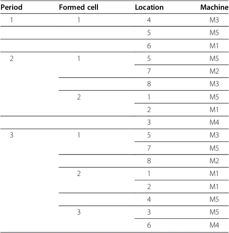
At the following two other numerical examples, three periods are presented to illustrate more the effect of variability in the number of formed cells on the perfor-mance of the developed model. The main difference be-tween these examples and the first one is that those later examples contain three planning periods. The data re-lated to the part demand in three periods for the second example is given in Table 7. Tables 8 and 9 show the cell configurations and the objective function value obtained for the second example, respectively.
As part demand increases in three periods, the num-ber of purchased machines and formed cells are in-creased to enhance process capacity due to meet the increased part demands. As can be seen, the number of formed cells in successive periods is 1, 2, and 3. In the first period, one duplicate of machines of types 1, 3, and 5 is purchased, assigned to cell 1, and located in loca-tions 6, 4, and 5, respectively. In the second period, one duplicate of machines of types 2, 4, and 5 is purchased and added to cells. Finally, in the third period, one dupli-cate of machines of types 1 and 5 is purchased. Average utilizations of machine time capacity in periods 1, 2, and 3 are 52%, 75%, and 93%, respectively. As it is expected, by increasing part demands, the machine utilization is heightened.
Part-related costs consist of intra-cell and inter-cell ma-terial handling costs. In addition, machine-related costs include costs of relocation, purchasing, overhead, and pro-cessing. If the number of formed cells had not been allowed to be changed in each period, three cells should have been formed. This could have totally led to forming nine cells in three periods and enforced forming cell cost as equal as 3 × 3 × 20,000 = 180,000. Therefore, the OFV would have been increased up to 452,261 (i.e., (452,261− 392,261) / 392,261 = 15%). To conclude, forming cells in changeable numbers makes the model enable to reduce the forming cell costs and the OFV.
Table 5 Optimal OFV and cost components for the example with three cells
OFV Intra-cell movement
Inter-cell movement
Machine relocation
Purchasing machine
Machine overhead
Processing machine
Forming cell
307,904.1 13,800 0 3,700 114,000 21,300 35,104.1 120,000
Table 6 Optimal OFV and cost components for the example with two cells
OFV Intra-cell movement
Inter-cell movement
Machine relocation
Purchasing machine
Machine overhead
Processing machine
Forming cell
252,812.7 19,695 0 2,350 94,000 18,800 37,967.7 80,000
Kiaet al. Journal of Industrial Engineering International2013,9:8 Page 9 of 14
The third example is presented by incorporating a ma-chine depot feature into the main model to keep idle machines in successive periods with completely different levels of part demands. This decreases machine overhead costs and provides empty locations to accommodate re-quired machines and configure cells more effectively. By considering machine depot, in each period that there is surplus capacity, idle machines can be removed from the cells and transferred to the machine depot. In addition, whenever it is necessary to increase the processing time capacity of the system because of high demand volume, those machines can be returned to the cells.
To define this feature, additional decision variables should be added to the mail model as follows:
Nmtþ number of machine type m removed from the ma-chine depot and returned to cells in periodt
N−
mt number of machine type m removed from cells
and moved to the machine depot in periodt
Also, constraint (4) should be modified by
∑
In addition, Constraint (15) needs to be added to the main model.
Equation (14) describes that the number of machine type
mutilized in the periodtis equal to the number of utilized machines of the same type in the previous period plus the number of new machines of the same type purchased at the beginning of the current period, plus the number of ma-chines of the same type removed from the machine depot and returned to the cells or minus the number of machines of the same type removed from the cells and moved to the machine depot at the beginning of the current period. In-equality (15) ensures that the number of machine type m
returned from the machine depot to the cells does not ex-ceed from the number of machine typem available in the machine depot in each period. It is worth mentioning that returning machines from the machine depot to cells can be started in the third period, because before that period there is any machines in the machine depot.
Now, the third numerical example with three periods is presented to illustrate the simultaneous effect of machine depot and variable cell number on the performance of the main model. The data related to the part demand for the third example is given in Table 10. The main difference between the first and third example is that the former contains three planning periods and six locations.
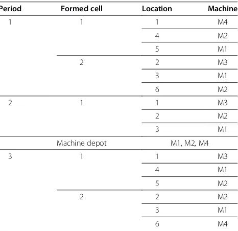
Table 11 shows the cell configurations and machine assignments to the formed cells and the machine depot for three periods. Also, the objective function value is presented in Table 12. Because of a high variation in de-mand of four parts in three periods, cell configurations are significantly different from each other in three periods. As it can be seen, in the first period, cells 1 and 2 are formed to process the part operations. In the first period, two units of machine types 1 and 2 and one unit of ma-chine types 3 and 4 are purchased and assigned to cells. For instance, one unit of machine types 1, 2, and 4 is assigned to cell 1 and one unit of machine types 1, 2, and 3 is assigned to cell 2. In the second period, cell 2 is eliminated to decrease manufacturing capacity of the system due to the reduced demand. In fact, one unit of machine types 1, 2, and 4 is removed from the system and transferred to the machine depot. Placing idle machines in a depot enables the model to reduce machine overhead costs, decrease the forming cell cost by closing underutilized cells, and provide empty locations to accommodate the required machines to
Table 7 Part demand for the second example
Period Part
1 2 3 4
1 0 200 0 300
2 600 800 0 0
3 400 700 600 500
Table 8 Cell configurations for the second example
Period Formed cell Location Machine
1 1 4 M3
Table 9 Optimal OFV for the second example
OFV Part-related
process new part demands. In the third period, machine types 1, 2, and 4 transferred to a machine depot in period 2 are returned to the system, and cell 2 is again formed to in-crease the manufacturing capacity in period 3.
The obtained solution for this example reveals the simul-taneous effect of the machine depot and variable cell num-ber on the performance of the main model. If this model is allowed to remove idle machines from the formed cells, it will eliminate machines M1, M2, and M4 from cells and keep them in the machine depot to reduce the overhead cost. In addition, keeping idle machines in a depot gives the model an opportunity to form fewer cells and reduce re-lated cost. As a result, the cost saving attained by keeping idle machines in a depot and forming fewer cells for this example is equal to (1,800 + 1,500 + 1,700 + 20,000 = 25,000). This is a reduction in the OFV as (25,000 / 361,411.3 × 100 = 7%).
Finally, it is worth mentioning that considering the manufacturing attributes (e.g., alternative process routing, purchasing machine, duplicate machines, machine depot, lot splitting, flexible cell configuration, and varying num-ber of formed cells) brings the flexibility for the presented model to respond to any change in the part demand and product mix.
Numerical examples for a multi-objective model by
ɛ-constraint method
Now, to investigate the performance of the proposed multi-objective model, the previous numerical example presented in ‘Illustrative numerical examples for the single-objective model’section is solved by the epsilon-constrained method considering the two conflicting objectivesZ1andZ2
simul-taneously. In ɛ-constraint method, one of the objectives is considered as the main objective function and the rest of them are incorporated in the constraint part of the model, assuming bounds for them. Therefore, the problem is changed to the objective problem. Then this single-objective model is solved, while the bounds of the new constraints are parametrically changed and the efficient so-lutions of the problem are obtained.
Table 13 shows the total workload cell imbalance (Z2)
and the total cost values (Z1) for each non-dominated
solution. In addition, the comparison between the first objectiveZ1and the workload imbalances of cells in the
second objective Z2 reveals that there is a reverse
rela-tionship between objectivesZ1andZ2.
A particular solution can be selected depending on the system designer's decision. The designer may either select a configuration of cells requiring lower cost and more workload cell imbalance (i.e., solution 1) in case of reduc-tion of manufacturing cost, or the one with higher cost and lesser workload cell imbalance (i.e., solution 4) may be adopted when the workload has to be distributed evenly among the cells.
As shown in Table 13, the workloads assigned to cells are totally different in solution 1 and results in a high vol-ume of workload imbalance among cells. However, in so-lution 4 the workloads are distributed among cells evenly and this results in a workload imbalance as 49.3 h. To de-crease the workload cell imbalance from 800 to 49.3 h, the value of cost objectiveZ1 is increased from 260,114.2 to
269,627.7 units. This result is expected because distribut-ing workload among cells more evenly needs transferrdistribut-ing some operations from cells with workload higher than the average to those with workload less than the average. This incurs more movements including intra and inter-cell and increases material handling costs and finally total costs.
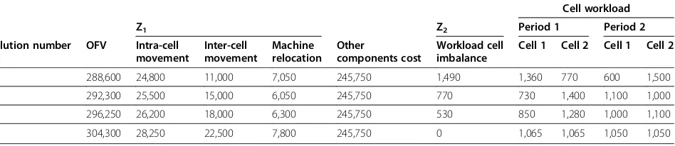
To say another instance that can be solved optimally in a reasonable time, the fourth numerical example is designed and solved where alternative process routings are eliminated from the main model due to reduce the compu-tational complexity. Table 14 presents four Pareto-optimal solutions obtained byɛ-constraint method. The cost com-ponents related to purchasing machine, machine overhead,
Table 10 Part demand for the third example
Period Part
1 2 3 4
1 140 680 250 650
2 170 210 0 290
3 280 220 730 370
Table 11 Cell configurations for the third example
Period Formed cell Location Machine
1 1 1 M4
4 M2
5 M1
2 2 M3
3 M1
6 M2
2 1 1 M3
2 M2
3 M1
Machine depot M1, M2, M4
3 1 1 M3
4 M1
5 M2
2 2 M2
3 M1
6 M4
Table 12 Optimal OFV for the third example
OFV Part-related cost
Machine-related cost
Forming cell cost
361,411.3 59,500 201,911.3 100,000
Kiaet al. Journal of Industrial Engineering International2013,9:8 Page 11 of 14
processing machine, and forming cell are 112,000, 24,600, 29,150, and 80,000 for all four Pareto solutions, respec-tively. Therefore, the sum of those components equal to 245,750 is shown in Table 14.
The trade-off between the optimal values ofZ1andZ2
shows a reverse relation, which is similar to the result observed in the previous example. As shown in Table 14, the workloads assigned to cells are totally different in so-lution 1 and results in a high volume of workload imbal-ance among cells. However, in solution 4, the workloads have distributed among cells evenly and this results in no workload imbalance. To decrease the workload cell imbalance from 1,490 h to 0, the value of cost objectiveZ1
is increased from 288,600 to 304,300 units. This result is expected because distributing workload among cells more evenly needs transferring some operations from cells with workload higher than average to those with workload less than average. That incurs more movements including intra- and inter-cellular and increases material handling costs and finally, total costs.
To the best of our knowledge, it is the first time that a multi-objective model integrating some important design features (e.g., alternative process routings, lot splitting, group layout, dynamic demands, and flexible reconfigu-ration in designing a CMS) is formulated. In comparison with the previous study (Kia et al. 2012), other improving features (e.g., a variable number of cells and balancing cell workload) are incorporated to the multi-objective inte-grated model in order to enhance its performance and re-duce the total costs as shown by a numerical example in ‘Illustrative numerical examples for the single-objective model’section.
Conclusion
This paper has presented a multi-objective mixed-integer nonlinear model that integrates the CF and group layout (GL) decisions in a dynamic environment. The presented model has combined a large design features introduced in the previous studies, such as alternative process routings, operation sequence, processing time, production volume of parts, purchasing machine, duplicate machines, ma-chine capacity, lot splitting, group layout, multi-rows lay-out of equal area facilities, and flexible reconfiguration. Additionally, it has addressed other important design fea-tures including a variable number of cells and balancing cell workload. The effect of newly integrated design fea-tures on improving the performance of the extended model has been illustrated by two numerical examples. The obtained results were revealed that the variable num-ber of cells could considerably improve the performance of the extended model by reducing the forming cell cost.
The extended model was capable in determining opti-mally the production volume of alternative processing routes of each part, the material flow happening between different machines, the cell configuration, the machine locations, the number of formed cells, and the number of purchased machines. Also, the model has been capable to distribute the workload among formed cells more evenly by scarifying other cost components, such as inter-cell material handling cost.
As it could be recognized by a huge amount of time spent to find optimal solutions for the presented examples, the presented model is NP-hardness. Hence, designing an effi-cient solution approach (e.g., meta-heuristics) is needed to solve large-sized problems. This is left to the future work.
Table 13 Pareto front obtained byɛ-constraint method for the first example with two objective functions
Solution number Z1 Z2
OFV Intra-cell movement
Inter-cell movement
Machine relocation
Purchasing machine
Machine overhead
Processing machine
Forming cell Workload cell imbalance
1 260,114.2 26,600 0 4,000 94,000 18,800 36,714.2 80,000 800
2 261,068.7 25,650 0 4,650 94,000 18,800 37,968.7 80,000 680
3 264,672.8 27,250 0 6,150 94,000 18,800 38,472.8 80,000 400
4 269,627.7 24,550 9,500 3,950 94,000 18,800 38,827.7 80,000 49.3
Table 14 Pareto optimal front obtained by∈-constraint method for the fourth example
Cell workload Z1 Z2 Period 1 Period 2
Solution number OFV Intra-cell movement
Inter-cell movement
Machine relocation
Other
components cost
Workload cell imbalance
Cell 1 Cell 2 Cell 1 Cell 2
1 288,600 24,800 11,000 7,050 245,750 1,490 1,360 770 600 1,500
2 292,300 25,500 15,000 6,050 245,750 770 730 1,400 1,100 1,000
3 296,250 26,200 18,000 6,300 245,750 530 850 1,280 1,000 1,100
Competing interests
The authors declare that they have no competing interests.
Authors' contributions
RK carried out the literature review studies, designed the mathematical model, and drafted the manuscript. HS participated in the design of the mathematical model and performed the numerical experiments. NJ and RTM conceived of the study and participated in its design and coordination. All authors read and approved the final manuscript.
Authors' information
RK is a Ph.D. candidate of Industrial Engineering (IE) at the Mazandaran University of Science & Technology, Babol, and a faculty member of Industrial Engineering Department in Islamic Azad University, Firoozkooh Branch. Research interests include design of cellular manufacturing systems, meta-heuristics, simulation modeling, facility design, mathematical modeling and optimization, fuzzy computing in more than 20 papers in international conferences and more than ten papers in international journals. HS is a faculty member of the Industrial Management Department in Islamic Azad University, Qom Branch. Also, HS teaches several courses in different branches of Islamic Azad University. Research interests include technology management, facility design, inventory control, and production planning. NJ is a faculty member of Industrial Engineering Department at Mazandran University of Science and Technology. He received his Ph.D. degree in Industrial Engineering from Iranian University of Science & Technology. Research interests include operation research, cellular manufacturing systems, decision making, fuzzy sets theory, and meta-heuristics. He has published articles in some journals such as Computers & Industrial Engineering, Expert Systems with Applications, Computers & Operations Research, Applied Soft Computing, International Journal of Advanced Manufacturing Technology, and Annals of Operations Research, RTM is a professor of Industrial Engineering at College of Engineering, University of Tehran in Iran. He obtained his Ph.D. in Industrial Engineering from the Swinburne University of Technology in Melbourne (1998), his M.Sc. in Industrial Engineering from the University of Melbourne in Melbourne (1994), and his B.Sc. in Industrial Engineering from the Iran University of Science & Technology in Tehran (1989). He serves as a member of the editorial boards of the International Journal of Engineering and Iranian Journal of Operations Research. He is also the Executive Member of the Board of Iranian Operations Research Society. He is the recipient of the 2009 and 2011 Distinguished Researcher Award and the 2010 Distinguished Applied Research Award at the University of Tehran, Iran. He has been selected as National Iranian Distinguished Researcher for 2008 and 2010. Prof. RTM has published three books, 12 book chapters, and more than 560 papers in reputable academic journals and conferences.
Acknowledgments
This work was financially supported by Islamic Azad University, Qom Branch, grant number 12006. The authors would like to sincerely thank the anonymous referees for their thorough reviews of the early versions of this paper and their very valuable comments.
Author details
1
Department of Industrial Engineering, Firoozkooh Branch,
Islamic Azad University, P.O. Box 148, Firoozkooh, Iran.2Department of Industrial Management, Qom Branch, Islamic Azad University, P.O. Box 3749113191, Qom, Iran.3Department of Industrial Engineering, Mazandaran University of Science and Technology, P.O. Box 734, Babol, Iran.4Department of Industrial Engineering, College of Engineering, University of Tehran, P.O. Box 11155-4563, Tehran, Iran.
Received: 15 August 2012 Accepted: 11 March 2013 Published: 25 April 2013
References
Ahkioon S, Bulgak AA, Bektas T (2009a) Integrated cellular manufacturing systems design with production planning and dynamic system reconfiguration. Eur J Oper Res 192:414–428
Ahkioon S, Bulgak AA, Bektas T (2009b) Cellular manufacturing systems design with routing flexibility, machine procurement, production planning and dynamic system reconfiguration. Int J Prod Res 47(6):1573–1600
Aramoon Bajestani M, Rabbani M, Rahimi-Vahed AR, Baharian Khoshkhou G (2009) A multi-objective scatter search for a dynamic cell formation problem. Comput Oper Res 36:777–794
Balakrishnan J, Cheng CH (2007) Multi-period planning and uncertainty issues in cellular manufacturing: a review and future directions. Eur J Oper Res 177:281–309
Baykasoglu A, Gindy NNZ, Cobb RC (2001) Capability based formulation and solution of multiple objective cell formation problems using simulated annealing. Integr Manuf Syst 12:258–274
Cao D, Chen M (2005) A robust cell formation approach for varying product demands. Int J of Prod Res 43(8):1587–1605
Collette Y, Siarry P (2003) Multiobjective optimization: principles and case studies. Springer, Berlin
Deljoo V, Mirzapour Al-e-hashem SMJ, Deljoo F, Aryanezhad MB (2010) Using genetic algorithm to solve dynamic cell formation problem. Appl Math Model 34(4):1078–1092
Drolet J, Marcoux Y, Abdulnour G (2008) Simulation-based performance comparison between dynamic cells, classical cells and job shops: a case study. Int J Prod Res 46(2):509–536
Defersha FM, Chen M (2008) A linear programming embedded genetic algorithm for an integrated cell formation and lot sizing considering product quality. Eur J Oper Res 187(1):46–69
Defersha FM, Chen M (2006) A comprehensive mathematical model for the design of cellular manufacturing systems. Int J Prod Econ 103:767–783 Ghotboddini MM, Rabbani M, Rahimian H (2011) A comprehensive dynamic cell
formation design: Benders' decomposition approach. Expert Syst Appl 38:2478–2488
Jolai F, Tavakkoli-Moghaddam R, Golmohammadi A, Javadi B (2012) An electromagnetism-like algorithm for cell formation and layout problem. Expert Syst Appl 39(2):2172–2182
Javadian N, Aghajani A, Rezaeian J, Ghaneian Sebdani MJ (2011) A multi-objective integrated cellular manufacturing systems design with dynamic system reconfiguration. Int J Adv Manuf Technol 56:307–317
Kia R, Baboli A, Javadian N, Tavakkoli-Moghaddam R, Kazemi M, Khorrami J (2012) Solving a group layout design model of a dynamic cellular manufacturing system with alternative process routings, lot splitting and flexible reconfiguration by simulated annealing. Comput Oper Res 39:2642–2658 Mahdavi I, Aalaei A, Paydar MM, Solimanpur M (2011) Multi-objective cell
formation and production planning in dynamic virtual cellular manufacturing systems. Int J Prod Res 49(21):6517–6537
Mahdavi I, Aalaei A, Paydar MM, Solimanpur M (2010) Designing a mathematical model for dynamic cellular manufacturing systems considering production planning and worker assignment. Comput Math Appl 60(4):1014–1025 Mungwattana A (2000) Design of cellular manufacturing systems for dynamic
and uncertain production requirements with presence of routing flexibility, Ph.D. Thesis. Polytechnic Institute and State University, Virginia
Nsakanda AL, Diaby M, Price WL (2006) Hybrid genetic approach for solving large-scale capacitated cell formation problems with multiple routings. Eur J Oper Res 171:1051–1070
Rafiee K, Rabbani M, Rafiei H, Rahimi-Vahed A (2011) A new approach towards integrated cell formation and inventory lot sizing in an unreliable cellular manufacturing system. Appl Math Model 35:1810–1819
Rezazadeh H, Mahini R, Zarei M (2011) Solving a dynamic virtual cell formation problem by linear programming embedded particle swarm optimization algorithm. Appl Soft Comput 11(3):3160–3169
Rheault M, Drolet J, Abdulnour G (1995) Physically reconfigurable virtual cells: a dynamic model for a highly dynamic environment. Comput Ind Eng 29(1–4):221–225
Saxena LK, Jain PK (2011) Dynamic cellular manufacturing systems design - a comprehensive model. Int J Adv Manuf Technol 53(1):11–34
Safaei N, Banjevic D, Jardine AKS (2010) Impact of the use-based maintenance policy on the performance of cellular manufacturing systems. Int J Prod Res 48(8):2233–2260
Safaei N, Tavakkoli-Moghaddam R (2009) Integrated multi-period cell formation and subcontracting production planning in dynamic cellular manufacturing. Int J Prod Res 120(2):301–314
Safaei N, Saidi-Mehrabad M, Jabal-Ameli MS (2008) A hybrid simulated annealing for solving an extended model of dynamic cellular manufacturing system. Eur J Oper Res 185:563–592
Solimanpur M, Vrat P, Shankar R (2004) Ant colony optimization algorithm to the inter-cell layout problem in cellular manufacturing. Eur J Oper Res 157:592–606
Kiaet al. Journal of Industrial Engineering International2013,9:8 Page 13 of 14
Wu X, Chu CH, Wang Y, Yan W (2007) A genetic algorithm for cellular manufacturing design and layout. Eur J Oper Res 181:156–167 Wemmerlov U, Johnson DJ (2000) Empirical findings in manufacturing cell
design. Int J Prod Res 38:481–507
Wemmerlov U, Hyer NL (1986) Procedures for the part family/machine group identification problem in cellular manufacture. J Oper Manag 6:125–147
doi:10.1186/2251-712X-9-8
Cite this article as:Kiaet al.:A multi-objective model for designing a group layout of a dynamic cellular manufacturing system.Journal of Industrial Engineering International20139:8.
Submit your manuscript to a
journal and benefi t from:
7Convenient online submission
7Rigorous peer review
7Immediate publication on acceptance
7Open access: articles freely available online
7High visibility within the fi eld
7Retaining the copyright to your article