Basic Concepts and Methods

(1)

(2)

CHEMICAL

THERMODYNAMICS

Basic Concepts and Methods

Seventh Edition

IRVING M. KLOTZ

Late Morrison Professor Emeritus, Northwestern University

ROBERT M. ROSENBERG

(3)

No part of this publication may be reproduced, stored in a retrieval system, or transmitted in any form or by any means, electronic, mechanical, photocopying, recording, scanning, or otherwise, except as permitted under Section 107 or 108 of the 1976 United States Copyright Act, without either the prior written permission of the Publisher, or authorization through payment of the appropriate per-copy fee to the Copyright Clearance Center, Inc., 222 Rosewood Drive, Danvers, MA 01923, (978) 750-8400, fax (978) 750-4470, or on the web at www.copyright.com. Requests to the Publisher for permission should be addressed to the Permissions Department, John Wiley & Sons, Inc., 111 River Street, Hoboken, NJ 07030, (201) 748-6011, fax (201) 748-6008, or online at http://www.wiley.com/go/permission. Limit of Liability/Disclaimer of Warranty: While the publisher and author have used their best efforts in preparing this book, they make no representations or warranties with respect to the accuracy or completeness of the contents of this book and specifically disclaim any implied warranties of merchantability or fitness for a particular purpose. No warranty may be created or extended by sales representatives or written sales materials. The advice and strategies contained herein may not be suitable for your situation. You should consult with a professional where appropriate. Neither the publisher nor author shall be liable for any loss of profit or any other commercial damages, including but not limited to special, incidental, consequential, or other damages.

For general information on our other products and services or for technical support, please contact our Customer Care Department within the United States at (800) 762-2974, outside the United States at (317) 572-3993 or fax (317) 572-4002.

Wiley also publishes it books in variety of electronic formats. Some content that appears in print may not be available in electronic formats. For more information about Wiley products, visit our web site at www.wiley.com.

Library of Congress Cataloging-in-Publication Data is available.

ISBN: 978-0-471-78015-1

(4)

Irving Myron Klotz January 22, 1916 – April 27, 2005

(5)

PREFACE

This is the seventh edition of a book that was ﬁrst published by Professor Klotz in 1950. He died while we were preparing this edition, and it is dedicated to his memory. Many friends have asked why a new edition of a thermodynamics text is necess-ary, because the subject has not changed basically since the work of J. Willard Gibbs. One answer is given by the statement of Lord Rayleigh in a letter to Gibbs,

The original version, though now attracting the attention it deserves, is too condensed and too difﬁcult for most, I might say all, readers.

This statement follows a request for Gibbs to prepare a new edition of, or a treatise founded on, the original. Those of us who still have difﬁculty with Gibbs are in good company. Planck wrote his famous textbook on thermodynamics independently of Gibbs, but subsequent authors were trying to make the work of Gibbs more easily understood than the Gibbs original. Similarly, each new edition of an established text tries to improve its pedagogical methods and bring itself up to date with recent developments or applications. This is the case with this edition.

One hundred fifty years ago, the two classic laws of thermodynamics were formu-lated independently by Kelvin and by Clausius, essentially by making the Carnot theorem and the Joule – Mayer – Helmholtz principle of conservation of energy con-cordant with each other. At first the physicists of the middle 1800s focused primarily on heat engines, in part because of the pressing need for efficient sources of power. At that time, chemists, who are rarely at ease with the calculus, shied away from

_{Quoted in E. B. Wilson,}_{Proc. Natl. Acad. Sci., U. S. A.}₃₁_{, 34 – 38 (1945).}

(18)

thermodynamics. In fact, most of them probably found the comment of the distin-guished philosopher and mathematician August Comte very congenial:

Every attempt to employ mathematical methods in the study of chemical questions must be considered profoundly irrational. If mathematical analysis should ever hold a promi-nent place in chemistry-an aberration which is happily impossible-it would occasion a rapid and widespread degradation of that science.

—A. Comte, Cours de philosophie positive, Bachelier, Paris, 1838, Vol. 3, pp. 28 – 29

By the turn of the nineteenth into the twentieth century, the work of Gibbs, Helmholtz, Planck, van’t Hoff, and others showed that the scope of thermodynamic concepts could be expanded into chemical systems and transformations. Consequently, during the ﬁrst 50 years of the twentieth century, thermodynamics progressively pervaded all aspects of chemistry and ﬂourished as a recognizable entity on its own—chemical thermodynamics.

By the middle of the twentieth century, biochemistry became increasingly under-stood in molecular and energetic terms, so thermodynamic concepts were extended into disciplines in the basic life sciences and their use has expanded progressively. During this same period, geology and materials science have adapted thermodyna-mics to their needs. Consequently, the successive revisions of this text incorporated examples and exercises representative of these ﬁelds.

In general, the spirit and format of the previous editions of this text have been maintained. The fundamental objective of the book remains unchanged: to present to the student the logical foundations and interrelationships of thermodynamics and to teach the student the methods by which the basic concepts may be applied to practical problems. In the treatment of basic concepts, we have adopted the classic, or phenomenological, approach to thermodynamics and have excluded the statistical viewpoint. This attitude has several pedagogical advantages. First, it permits the maintenance of a logical unity throughout the book. In addition, it offers an opportunity to stress the “operational” approach to abstract concepts. Furthermore, it makes some contribution toward freeing the student from a perpetual yearning for a mechanical analog for every new concept that is introduced.

A great deal of attention is paid in this text to training the student in the application of the basic concepts to problems that are commonly encountered by the chemist, the biologist, the geologist, and the materials scientist. The mathematical tools that are necessary for this purpose are considered in more detail than is usual. In addition, computational techniques, graphical, numerical, and analytical, are described fully and are used frequently, both in illustrative and in assigned problems. Furthermore, exercises have been designed to simulate more than in most texts the type of problem that may be encountered by the practicing scientist. Short, unrelated exer-cises are thus kept to a minimum, whereas series of computations or derivations, which illustrate a technique or principle of general applicability, are emphasized.

(19)

the fundamental principles and be shown how these can be applied to a few typical problems, that individual will be capable of examining other special topics indepen-dently or with the aid of one of the excellent comprehensive treatises that are available.

Another feature of this book is the extensive use of subheadings in outline form to indicate the position of a given topic in the general sequence of presentation. In using this method of presentation, we have been inﬂuenced strongly by the viewpoint expressed so aptly by Poincare:

The order in which these elements are placed is much more important than the elements themselves. If I have the feeling. . . of this order, so as to perceive at a glance the reason-ing as a whole, I need no longer fear lest I forget one of the elements, for each of them will take its allotted place in the array, and that without any effort of memory on my part. —H. Poincare, The Foundations of Science, translated by G. B. Halsted, Science Press, 1913.

It is a universal experience of teachers, that students can to retain a body of infor-mation much more effectively if they are aware of the place of the parts in the whole. Although thermodynamics has not changed fundamentally since the ﬁrst edition was published, conventions and pedagogical approaches have changed, and new applications continue to appear. A new edition prompts us to take note of the pro-gressive expansion in range of areas in science and engineering that have been illuminated by thermodynamic concepts and principles. We have taken the opportu-nity, therefore, to revise our approach to some topics and to add problems that reﬂect new applications. We have continued to take advantage of the resources available on the World Wide Web so that students can gain access to databases available online. We are indebted to the staff of Seeley-Mudd Science and Engineering Library for their assistance in obtaining resource materials. R.M.R. is grateful to the Chemistry Department of Northwestern University for its hospitality during his extended visit-ing appointment. We thank Warren Peticolas for his comments on several chapters and for his helpful suggestions on Henry’s law. We are grateful to E. Virginia Hobbs for the index and to Sheree Van Vreede for her copyediting. We thank Rubin Battino for his careful reading of the entire manuscript.

A solutions manual that contains solutions to most exercises in the text is available.

While this edition was being prepared, the senior author, Irving M. Klotz, died. He will be sorely missed by colleagues, students, and the scientiﬁc community. This edition is dedicated to his memory.

ROBERTM. ROSENBERG

Evanston, Illinois

(20)

(21)

CHAPTER 1 INTRODUCTION

1.1 ORIGINS OF CHEMICAL THERMODYNAMICS

An alert young scientist with only an elementary background in his or her field might be surprised to learn that a subject called “thermodynamics” has any relevance to chemistry, biology, material science, and geology. The term thermodynamics, when taken literally, implies a field concerned with the mechanical action produced by heat. Lord Kelvin invented the name to direct attention to thedynamicnature of heatand to contrast this perspective with previous conceptions of heat as a type of fluid. The name has remained, although the applications of the science are much broader than when Kelvin created its name.

In contrast to mechanics, electromagnetic ﬁeld theory, or relativity, where the names of Newton, Maxwell, and Einstein stand out uniquely, the foundations of thermodynamics originated from the thinking of over half a dozen individuals: Carnot, Mayer, Joule, Helmholtz, Rankine, Kelvin, and Clausius [1]. Each person provided crucial steps that led to the grand synthesis of the two classic laws of thermodynamics.

Eighteenth-century and early nineteenth-century views of the nature of heat were founded on the principle of conservation of caloric. This principle is an eminently attractive basis for rationalizing simple observations such as temperature changes that occur when a cold object is placed in contact with a hot one. The cold object seems to have extracted something (caloric) from the hot one. Furthermore,

Chemical Thermodynamics: Basic Concepts and Methods, Seventh Edition. By Irving M. Klotz and Robert M. Rosenberg

Copyright#2008 John Wiley & Sons, Inc.

(22)

if both objects are constituted of the same material, and the cold object has twice the mass of the hot one, then we observe that the increase in temperature of the former is only half the decrease in temperature of the latter. A conservation principle develops naturally. From this principle, the notion of the ﬂow of a substance from the hot to the cold object appears almost intuitively, together with the concept that the total quantity of the caloric can be represented by the product of the mass mul-tiplied by the temperature change. With these ideas in mind, Black was led to the discovery of speciﬁc heat, heat of fusion, and heat of vaporization. Such successes established the concept of caloric so solidly and persuasively that it blinded even the greatest scientists of the early nineteenth century. Thus, they missed seeing well-known facts that were common knowledge even in primitive cultures, for example, that heat can be produced by friction. It seems clear that the earliest of the founders of thermodynamics, Carnot, accepted conservation of caloric as a basic axiom in his analysis [2] of the heat engine (although a few individuals [3] claim to see an important distinction in the contexts of Carnot’s uses of “calorique” versus “chaleur”).

Although Carnot’s primary objective was to evaluate the mechanical efﬁciency of a steam engine, his analysis introduced certain broad concepts whose signiﬁcance goes far beyond engineering problems. One of these concepts is the reversible process, which provides for thermodynamics the corresponding idealization that “frictionless motion” contributes to mechanics. The idea of “reversibility” has appli-cability much beyond ideal heat engines. Furthermore, it introduces continuity into the visualization of the process being considered; hence, it invites the introduction of the differential calculus. It was Clapeyron [4] who actually expounded Carnot’s ideas in the notation of calculus and who thereby derived the vapor pressure equation associated with his name as well as the performance characteristics of ideal engines. Carnot also leaned strongly on the analogy between a heat engine and a hydro-dynamic one (the water wheel) for, as he said:

we can reasonably compare the motive power of heat with that of a head of water.

(23)

When faced in the late 1840s with the idea of conservation of (heat plus work) proposed by Joule, Helmholtz, and Mayer, Kelvin at ﬁrst rejected it (as did the Proceedings of the Royal Society when presented with one of Joule’s manuscripts) because conservation of energy (work plus heat) was inconsistent with the Carnot analysis of the fall of an unchanged quantity of heat through an ideal thermal engine to produce work. Ultimately, however, between 1849 and 1851, Kelvin and Clausius, each reading the other’s papers closely, came to recognize that Joule and Carnot could be made concordant if it was assumed that onlypartof the heat entering the Carnot engine at the high temperature was released at the lower level and that the difference was converted into work. Clausius was the ﬁrst to express this in print. Within the next few years, Kelvin developed the mathematical expression SQ/T¼0 for “the second fundamental law of the dynamical theory of heat” and

began to use the word thermodynamic, which he had actually coined earlier. Clausius’s analysis [5] led him, in turn, to the mathematical formulation of Ð

dQ/T0 for the second law; in addition, he invented the term entropy (as an alternative to Kelvin’s “dissipation of energy”), for, as he says,

I hold it better to borrow terms for important magnitudes from the ancient languages so that they may be adopted unchanged in all modern languages.

Thereafter, many individuals proceeded to show that the two fundamental laws, explicitly so-called by Clausius and Kelvin, were applicable to all types of macro-scopic natural phenomena and not just to heat engines. During the latter part of the nineteenth century, then, the scope of thermodynamics widened greatly. It became apparent that the same concepts that allow one to predict the maximum efﬁciency of a heat engine apply to other energy transformations, including transformations in chemical, biological, and geological systems in which an energy change is not obvious. For example, thermodynamic principles permit the computation of the maximum yield in the synthesis of ammonia from nitrogen and hydrogen under a variety of conditions of temperature and pressure, with important consequences to the chemical fertilizer industry. Similarly, the equilibrium distribution of sodium and potassium ions between red blood cells and blood plasma can be calculated from thermodynamic relationships. It was the observation of deviations from an equi-librium distribution that led to a search for mechanisms of active transport of these alkali metal ions across the cell membrane. Also, thermodynamic calculations of the effect of temperature and pressure on the transformation between graphite and diamond have generated hypotheses about the geological conditions under which natural diamonds can be made.

For these and other phenomena, thermal and work quantities, although controlling factors, are only of indirect interest. Accordingly, a more reﬁned formulation of ther-modynamic principles was established, particularly by Gibbs [6] and, later, indepen-dently by Planck [7], that emphasized the nature and use of several special functions or potentials to describe the state of a system. These functions have proved convenient and powerful in prescribing the rules that govern chemical and physical transitions. Therefore, in a sense, the name “energetics” is more descriptive than is

(24)

“thermodynamics” insofar as applications to chemistry are concerned. More commonly, one afﬁxes the adjective “chemical” to thermodynamics to indicate the change in emphasis and to modify the literal and original meaning of thermodynamics.

1.2 OBJECTIVES OF CHEMICAL THERMODYNAMICS

In practice, the primary objective of chemical thermodynamics is to establish a cri-terion for determining the feasibility or spontaneity of a given physical or chemical transformation. For example, we may be interested in a criterion for determining the feasibility of a spontaneous transformation from one phase to another, such as the conversion of graphite to diamond, or the spontaneous direction of a metabolic reaction that occurs in a cell. On the basis of the ﬁrst and second laws of thermodyn-amics, which are expressed in terms of Gibbs’s functions, several additional theoreti-cal concepts and mathematitheoreti-cal functions have been developed that provide a powerful approach to the solution of these questions.

Once the spontaneous direction of a natural process is determined, we may wish to know how far the process will proceed before reaching equilibrium. For example, we might want to ﬁnd the maximum yield of an industrial process, the equilibrium solu-bility of atmospheric carbon dioxide in natural waters, or the equilibrium concen-tration of a group of metabolites in a cell. Thermodynamic methods provide the mathematical relations required to estimate such quantities.

Although the main objective of chemical thermodynamics is the analysis of spon-taneity and equilibrium, the methods also are applicable to many other problems. For example, the study of phase equilibria, in ideal and nonideal systems, is basic to the intelligent use of the techniques of extraction, distillation, and crystallization; to met-allurgical operations; to the development of new materials; and to the understanding of the species of minerals found in geological systems. Similarly, the energy changes that accompany a physical or chemical transformation, in the form of either heat or work, are of great interest, whether the transformation is the combustion of a fuel, the ﬁssion of a uranium nucleus, or the transport of a metabolite against a concen-tration gradient. Thermodynamic concepts and methods provide a powerful approach to the understanding of such problems.

1.3 LIMITATIONS OF CLASSIC THERMODYNAMICS

Although descriptions of chemical change are permeated with the terms and language of molecular theory, the concepts of classic thermodynamics are independent of mole-cular theory; thus, these concepts do not require modiﬁcation as our knowledge of molecular structure changes. This feature is an advantage in a formal sense, but it is also a distinct limitation because we cannot obtain information at a molecular level from classic thermodynamics.

(25)

magnetic susceptibility, and heat capacity). It is an empirical and phenomenological science, and in this sense, it resembles classic mechanics. The latter also is concerned with the behavior of macroscopic systems, with the position and the velocity of a body as a function of time, without regard to the body’s molecular nature.

Statistical mechanics(orstatistical thermodynamics) is the science that relates the properties of individual molecules and their interactions to the empirical results of classical thermodynamics. The laws of classic and quantum mechanics are applied to molecules; then, by suitable statistical averaging methods, the rules of macroscopic behavior that would be expected from an assembly of many such molecules are for-mulated. Because classical thermodynamic results are compared with statistical averages over very large numbers of molecules, it is not surprising that fluctuation phenomena, such as Brownian motion, the “shot effect,” or certain turbidity pheno-mena, cannot be treated by classical thermodynamics. Now we recognize that all such phenomena are expressions of local microscopic fluctuations in the behavior of a rela-tively few molecules that deviate randomly from the average behavior of the entire assembly. In this submicroscopic region, such random fluctuations make it impossi-ble to assign a definite value to properties such as temperature or pressure. However, classical thermodynamics is predicated on the assumption that a definite and repro-ducible value always can be measured for such properties.

In addition to these formal limitations, limitations of a more functional nature also exist. Although the concepts of thermodynamics provide the foundation for the solu-tion of many chemical problems, the answers obtained generally are not definitive. Using the language of the mathematician, we might say that classical thermodynamics can formulatenecessaryconditions but notsufficientconditions. Thus, a thermodyn-amic analysis may rule out a given reaction for the synthesis of some substance by indi-cating that such a transformation cannot proceed spontaneously under any set of available conditions. In such a case, we have a definitive answer. However, if the analy-sis indicates that a reaction may proceed spontaneously, no statement can be made from classical thermodynamics alone indicating that it will do so in any finite time.

For example, classic thermodynamic methods predict that the maximum equili-brium yield of ammonia from nitrogen and hydrogen is obtained at low temperatures. Yet, under these optimum thermodynamic conditions, the rate of reaction is so slow that the process is not practical for industrial use. Thus, a smaller equilibrium yield at high temperature must be accepted to obtain a suitable reaction rate. However, although the thermodynamic calculations provide no assurance that an equilibrium yield will be obtained in a ﬁnite time, it was as a result of such calculations for the synthesis of ammonia that an intensive search was made for a catalyst that would allow equilibrium to be reached.

Similarly, specific catalysts called enzymes are important factors in determining what reactions occur at an appreciable rate in biological systems. For example, ade-nosine triphosphate is thermodynamically unstable in aqueous solution with respect to hydrolysis to adenosine diphosphate and inorganic phosphate. Yet this reaction proceeds very slowly in the absence of the specific enzyme adenosine triphosphatase. This combination of thermodynamic control of direction and enzyme control of rate makes possible the finely balanced system that is a living cell.

(26)

In the case of the graphite-to-diamond transformation, thermodynamic results predict that graphite is the stable allotrope at a ﬁxed temperature at all pressures below the transition pressure and that diamond is the stable allotrope at all pressures above the transition pressure. But diamond is not converted to graphite at low press-ures for kinetic reasons. Similarly, at conditions at which diamond is the thermody-namically stable phase, diamond can be obtained from graphite only in a narrow temperature range just below the transition temperature, and then only with a catalyst or at a pressure sufﬁciently high that the transition temperature is about 2000 K.

Just as thermodynamic methods provide only alimiting value for the yield of a chemical reaction, so also do they provide only a limiting value for the work obtain-able from a chemical or physical transformation. Thermodynamic functions predict the work that may be obtained if the reaction is carried out with inﬁnite slowness, in a so-called reversible manner. However, it is impossible to specify the actual work obtained in a real or natural process in which the time interval is ﬁnite. We can state, nevertheless, that the real work will be less than the work obtainable in a reversible situation.

For example, thermodynamic calculations will provide a value for themaximum voltage of a storage battery—that is, the voltage that is obtained when no current is drawn. When current is drawn, we can predict that the voltage will be less than the maximum value, but we cannot predict how much less. Similarly, we can calcu-late themaximumamount of heat that can be transferred from a cold environment into a building by the expenditure of a certain amount of work in a heat pump, but the actual performance will be less satisfactory. Given a nonequilibrium distribution of ions across a cell membrane, we can calculate theminimumwork required to maintain such a distribution. However, the actual process that occurs in the cell requires much more work than the calculated value because the process is carried out irreversibly. Although classical thermodynamics can treat only limiting cases, such a restriction is not nearly as severe as it may seem at ﬁrst glance. In many cases, it is possible to approach equilibrium very closely, and the thermodynamic quantities coincide with actual values, within experimental error. In other situations, thermodynamic analysis may rule out certain reactions under any conditions, and a great deal of time and effort can be saved. Even in their most constrained applications, such as limiting solutions within certain boundary values, thermodynamic methods can reduce materially the amount of experimental work necessary to yield a deﬁnitive answer to a particular problem.

REFERENCES

1. D. S. L. Cardwell, From Watt to Clausius: The Rise of Thermodynamics in the Early Industrial Age, Cornell University Press, Ithaca, NY, 1971.

(27)

3. H. L. Callendar,Proc. Phys. Soc. (London)23, 153 (1911); V. LaMer,Am. J. Phys.23, 95 (1955).

4. E. Clapeyron,J. Ecole Polytech. (Paris)14, 153 (1834); Mendoza,Motive Power of Fire. 5. R. Clausius,Pogg. Ann. Series III79, 368, 500 (1859);Series V5, 353 (1859);Ann. Phys.

125, 353 (1865); Mendoza,Motive Power of Fire.

6. J. W. Gibbs,Trans. Conn. Acad. Sci.3, 228 (1876);The Collected Works of J Willard Gibbs, Yale University Press, New Haven, CT, 1928; reprinted 1957.

7. M. Planck,Treatise on Thermodynamics, Berlin, 1897, Translated from the seventh German edition, Dover Publications, New York; M. Born,Obituary Notices of Fellows of the Royal Society,6, 161 (1948).

(28)

(29)

CHAPTER 2 MATHEMATICAL PREPARATION

FOR THERMODYNAMICS

Ordinary language is deficient in varying degrees for expressing the ideas and findings of science. An exact science must be founded on precise definitions that are difficult to obtain by verbalization. Mathematics, however, offers a precise mode of expression. Mathematics also provides a rigorous logical procedure and a device for the development in succinct form of a long and often complicated argu-ment. A long train of abstract thought can be condensed with full preservation of con-tinuity into brief mathematical notation; thus, we can proceed readily with additional steps in reasoning without carrying in our minds the otherwise overwhelming burden of all previous steps in the sequence. Yet, we must be able to express the results of our investigations in plain language if we are to communicate our results to a general audience.

Most branches of theoretical science can be expounded at various levels of abstrac-tion. The most elegant and formal approach to thermodynamics, that of Caratheodory [1], depends on a familiarity with a special type of differential equation (Pfaff equation) with which the usual student of chemistry is unacquainted. However, an introductory presentation of thermodynamics follows best along historical lines of development, for which only the elementary principles of calculus are necessary. We follow this approach here. Nevertheless, we also discuss exact differentials and Euler’s theorem, because many concepts and derivations can be presented in a more satisfying and precise manner with their use.

Chemical Thermodynamics: Basic Concepts and Methods, Seventh Edition. By Irving M. Klotz and Robert M. Rosenberg

Copyright#2008 John Wiley & Sons, Inc.

(30)

2.1 VARIABLES OF THERMODYNAMICS

Extensive and Intensive Quantities [2]

In the study of thermodynamics we can distinguish between variables that are inde-pendent of the quantity of matter in a system, theintensive variables, and variables that depend on the quantity of matter. Of the latter group, those variables whose values are directly proportional to the quantity of matter are of particular interest and are simple to deal with mathematically. They are called extensive variables. Volume and heat capacity are typical examples ofextensivevariables, whereas temp-erature, pressure, viscosity, concentration, and molar heat capacity are examples of intensivevariables.

Units and Conversion Factors

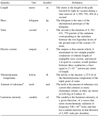
The base units of measurement under the Systeme International d’Unites, or SI units, are given in Table 2.1 [3].

Some SI-derived units with special names are included in Table 2.2. The standard atmosphere may be used temporarily with SI units; it is defined to be equal to 1.01325105Pa. The thermochemical calorie is no longer recommended as a unit of energy, but it is defined in terms of an SI unit, joules, symbol J, as 4.184 J [4]. The unit of volume, liter, symbol L, is now defined as 1 dm3.

The authoritative values for physical constants and conversion factors used in thermodynamic calculations are assembled in Table 2.3. Furthermore, information about the proper use of physical quantities, units, and symbols can be found in several additional sources [5].

2.2 ANALYTIC METHODS

Partial Differentiation

As the state of a thermodynamic system generally is a function of more than one inde-pendent variable, it is necessary to consider the mathematical techniques for expres-sing these relationships. Many thermodynamic problems involve only two independent variables, and the extension to more variables is generally obvious, so we will limit our illustrations to functions of two variables.

Equation for the Total Differential. Let us consider a speciﬁc example: the volume of a pure substance. The molar volumeVmis a functionfonly of the

tempe-rature T and pressure P of the substance; thus, the relationship can be written in general notation as

(31)

in which the subscript “m” indicates a molar quantity. Using the principles of calcu-lus [6], we can write for the total differential

dVm¼

TABLE 2.1. Base SI Unitsa

Quantity Unit Symbol Deﬁnition

Length meter m The meter is the length of the path

traveled by light in vacuum during a time interval of 1/299, 792, 458 of a second.

Mass kilogram kg The kilogram is the mass of the

international prototype of the kilogram.

Time second s The second is the duration of 9, 192,

631, 770 periods of the radiation corresponding to the transition between the two hyperﬁne levels of the ground state of the cesium-133 atom.

Electric current ampere A The ampere is that current which, if

maintained in two straight parallel conductors of inﬁnite length of negligible cross section, and placed 1 m apart in vacuum, would produce between these conductors a force equal to 21027_{newton per meter}

of length. Thermodynamic

temperature

kelvin K The kelvin is the fraction 1/273.16 of the thermodynamic temperature of the triple point of water.

Amount of substanceb mole mol The mole is the amount of substance of a system that contains as many elementary entities as there are atoms in 0.012 kg of Carbon 12.

Luminous intensity candela cd The candela is the luminous intensity, in a given direction, of a source that emits monochromatic radiation of frequency 5401012hertz and that has a radiant intensity in that direction of 1/683 watts per steradian.

a_{B. N. Taylor,}_{Guide to the Use of the International System of Units (SI)}_{, NIST Special Publication 811,}

Gaithersburg, MD, 1995. http://www.physics.nist.gov/cuu/units/current.html. http://www.bpim.fr.

b_{The amount of substance should be expressed in units of moles, with one mole being Avogadro’s constant}

number of designated particles or groups of particles, whether these are electrons, atoms, molecules, or the number of molecules of reactants and products speciﬁed by a chemical equation.

(32)

For the special case of one mole of an ideal gas, Equation (2.1) becomes

where R is the universal gas constant. As the partial derivatives are given by the expressions

Energy, work, quantity of heat joule J N m

Power watt W J s21

Electric charge coulomb C A s

Electric potential, electromotive

Heat capacity, entropy joule per

kelvin

J K21

TABLE 2.3. Fundamental Constants and Conversion Factors

Ice-point temperature, (08C) ¼273.15 Kelvins (K)

Gas constant,R ¼8.314471 J K21mol21(+15)a

a_{2002 CODATA recommended values of the Fundamental Physical Constants, ICSU-CODATA Task}

Group on Fundamental Constants, P. J. Mohr and B. N. Taylor,Rev. Mod. Phys.,77, 1 (2005). (http://physics. nist.gov/cuu/Constants). Uncertainties are in the last two digits of each value.

(33)

and

the total differential for the special case of the ideal gas can be obtained by substituting from Equations (2.4) and (2.5) into Equation (2.2) and is given by the relationship

We shall have frequent occasion to use this expression.

Conversion Formulas. Often no convenient experimental method exists for evaluating a derivative needed for the numerical solution of a problem. In this case we must convert the partial derivative to relate it to other quantities that are readily available. The key to obtaining an expression for a particular partial derivative is to start with the total derivative for the dependent variable and to realize that a derivative can be obtained as the ratio of two differentials [8]. For example, let us convert the derivatives of the volume function discussed in the preceding section.

1. We can obtain a formula for (@P/@T)Vby using Equation (2.2) for the total differential of V as a function of T and P and dividing both sides by dT. Keeping in mind thatdVm¼0, we obtain

Now, if we indicate explicitly for the second factor of the ﬁrst term on the right side thatVmis constant, and if we rearrange terms, we obtain

@P evaluation, we could establish its value from the more readily measurable (@Vm/@P)T and (@Vm/@T)P. These coefﬁcients are related to the coefﬁcient

of thermal expansiona, (1/V)(@V/@T)Pand to thecoefﬁcient of

compressibi-lityb,2(1/V)(@V/@P)T.

We can verify the validity of Equation (2.8) for an ideal gas by evaluating both sides explicitly and showing that the equality holds. The values of the

(34)

partial derivatives can be determined by reference to Equations (2.4) and (2.5), and the following deductions can be made:

@P ﬁnd dVm/dPand by imposing the restriction that Vmbe constant. Thus, we

obtain

3. From Equations (2.8) and (2.11), we infer a third relationship

@P

Thus, we see again that the derivatives can be manipulated practically as if they were fractions.

4. A fourth relationship is useful for problems in which a new independent vari-able is introduced. For example, we could consider the volumeVof a pure sub-stance as a function of pressure and energyU.

V ¼g(U,P)

We then may wish to evaluate the partial derivative (@Vm/@P)U that is, the change of volume with change in pressure at constant energy. A suitable expression for this derivative in terms of other partial derivatives can be obtained from Equation (2.2) by dividing dVm by dP and explicitly

(35)

5. A ﬁfth formula, for use in situations in which a new variableX(P,T) is to be introduced, is an example of the chain rule of differential calculus. The formula is

These illustrations, which are based on the example of the volume function, are typical of the type of conversion that is required so frequently in thermo-dynamic manipulations.

Exact Differentials

Many thermodynamic relationships can be derived easily by using the properties of the exact differential. As an introduction to the characteristics of exact differentials, we shall consider the properties of certain simple functions used in connection with a gravitational ﬁeld. We will use a capitalDto indicate an inexact differential, as inDW, and a smalldto indicate an exact differential, as indU.

Example of the Gravitational Field. Let us compare the change in potential energy and the work done in moving a large boulder up a hill against the force of gravity. From elementary physics, we see that these two quantities, DU and W, differ in the following respects.

1. The change in potential energy depends only on the initial and ﬁnal heights of the stone, whereas the work done (as well as the heat generated) depends on the path used. That is, the quantity of work expended if we use a pulley and tackle to raise the boulder directly will be much less than if we have to move the object up the hill by pushing it over a long, muddy, and tortuous road. However, the change in potential energy is the same for both paths as long as they have the same starting point and the same end point.

2. An explicit expression for the potential energyUexists, and this function can be differentiated to givedU, whereas no explicit expression forWthat leads to DW can be obtained. The function for the potential energy is a particularly simple one for the gravitational ﬁeld because two of the space coordinates drop out and only the heighthremains. That is,

U¼constantþmgh (2:15)

The symbols m andg have the usual signiﬁcance of mass and acceleration because of gravity, respectively.

3. A third difference betweenDUandWlies in the values obtained if one uses a cyclic path, as in moving the boulder up the hill and then back down to the

(36)

initial point. For such a cyclic or closed path, the net change in potential energy is zero because the ﬁnal and initial points are identical. This fact is represented by the equation

þ

dU¼0 (2:16)

in which Þ

denotes the integral around a closed path. However, the value of W for a complete cycle usually is not zero, and the value obtained depends on the particular cyclic path that is taken.

General Formulation. To understand the notation for exact differentials that gen-erally is adopted, we shall express the total differential of a general functionL(x,y) to indicate explicitly that the partial derivatives are functions of the independent vari-ables (xandy), and that the differential is a function of the independent variables and their differentials (dxanddy). That is,

dL(x,y,dx,dy)¼M(x,y)dxþN(x,y)dy (2:17) in which

M(x,y)¼ @L @x

y

(2:18) and

N(x,y)¼ @L @y

x

(2:19)

The notation in Equation (2.l7) makes explicit the notion that, in general,dLis a func-tion of the path chosen. Using this expression, we can summarize the characteristics of an exact differential as follows:

1. A functionf(x, y) exists, such that

df(x,y)¼dL(x,y,dx,dy) (2:20)

That is, the differential is a function only of the coordinates and is independent of the path.

2. The value of the integral over any speciﬁed path, that is, the line integral [7]

ð2

1

dL(x,y,dx,dy)¼

ð2

1

df(x,y) (2:21)

(37)

3. The line integral over a closed path is zero; that is,

þ

dL(x,y,dx,dy)¼

þ

df(x,y)¼0 (2:22)

It is this last characteristic that is used most frequently in testing thermodynamic functions for exactness. If the differentialdJof a thermodynamic quantityJis exact, thenJis called athermodynamic property or astate function.

Reciprocity Characteristic. A common test of exactness of a differential expressiondL(x, y, dx, dy)is whether the following relationship holds:

@

We can see that this relationship must be true ifdLis exact, because in that case a functionf(x, y)exists such that

dL(x,y,dx,dy)¼df(x,y)¼ @f

It follows from Equations (2.20) and (2.24) that

M(x,y)¼ @f

But, for the functionf(x,y), we know from the principles of calculus that

@

That is, the order of differentiation is immaterial for any function of two variables. Therefore, ifdLis exact, Equation (2.23) is correct [8].

To apply this criterion of exactness to a simple example, let us assume that we know only the expression for the total differential of the volume of an ideal gas [Equation (2.6)] and do not know whether this differential is exact. Applying

(38)

Equation (2.23) to Equation (2.6), we obtain

@ @P

R P

¼ R

P2¼

@ @T

RT P2

Thus, we would know that the volume of an ideal gas is a thermodynamic property, even if we had not been aware previously of an explicit function forVm.

Homogeneous Functions

In connection with the development of the thermodynamic concept of partial molar quantities, it is desirable to be familiar with a mathematical relationship known as Euler’s theorem.As this theorem is stated with reference to “homogeneous” func-tions, we will consider brieﬂy the nature of these functions.

Deﬁnition. As a simple example, let us consider the function

u¼ax2þbxyþcy2 (2:28)

If we replace the variablesxandybylxandly, in whichlis a parameter, we can write

u ¼u(lx,ly)¼a(lx)2þb(lx)(ly)þc(ly)2 ¼l2ax2þl2bxyþl2cy2

¼l2(ax2þbxyþcy2)

¼l2_u ₍₂_:₂₉₎

As the net result of multiplying each independent variable by the parameterlmerely has been to multiply the function byl2

, the function is calledhomogeneous.Because the exponent oflin the result is 2, the function is of thesecond degree.

Now we turn to an example of experimental signiﬁcance. If we mix certain quan-tities of benzene and toluene, which form an ideal solution, the total volumeVwill be given by the expression

V ¼V†

mbnbþVmt†nt (2:30)

in whichnbis the number of moles of benzene,V†mbis the volume of one mole of pure

benzene,ntis the number of moles of toluene, andV†mtis the volume of one mole of

pure toluene. Suppose that we increase the quantity of each of the independent vari-ables,nbandnt, by the same factor, say 2. We know from experience that the volume

(39)

replacenbbylnbandntbylnt, the new volumeV will be given by

V ¼V†

mblnbþVmt†lnt

¼l(V†

mbnbþVmt†nt)

¼lV (2:31)

The volume function then is homogeneous of the ﬁrst degree, because the parameter l, which factors out, occurs to the ﬁrst power. Although an ideal solution has been used in this illustration, Equation (2.31) is true of all solutions. However, for nonideal solutions, the partial molar volume must be used instead of molar volumes of the pure components (see Chapter 9).

Proceeding to a general deﬁnition, we can say that a function, f(x, y, z,. . .) is homogeneous of degree n if, upon replacement of each independent variable by an arbitrary parameter l times the variable, the function is multiplied by ln†_, that is, if

fðlx,ly,lz,. . .Þ ¼ln_f_ðx

,y,z,. . .Þ (2:32)

Euler’s Theorem. The statement of the theorem can be made as follows: Iff(x, y) is a homogeneous function of degreen, then

x @f @x

y þy @f

@y

x

¼nf(x,y) (2:33)

The proof can be carried out by the following steps. First let us represent the vari-ableslxandlyby

x ¼lx (2:34)

and

y ¼ly (2:35)

Then, becausef(x,y) is homogeneous

f¼f(x,y)¼f(lx,ly)¼ln_f₍_x_,_y₎ ₍₂_:₃₆₎

The total differentialdfis given by

df¼@f

@xdx _þ@f

@ydy

(2:37)

(40)

Hence

From Equations (2.34) and (2.35)

dx

dl ¼x (2:39)

and

dy

dl ¼y (2:40)

Consequently, Equation (2.38) can be rewritten as

df

Using the equalities in Equation (2.36) we can obtain

df

Equating the right sides of Equations (2.41) and (2.42), we obtain

x@f

Because l is an arbitrary parameter, Equation (2.43) must hold for any particular value. It must be true then forl¼1. In such an instance, Equation (2.43) reduces to

x @f

This equation is Euler’s theorem [Equation (2.33)].

As one example of the application of Euler’s theorem, we refer again to the volume of a two-component system. Evidently the total volume is a function of the number of moles of each component:

V ¼f(n1,n2) (2:44)

(41)

function of the ﬁrst degree is anextensive property. Applying Euler’s theorem, we

whereVm1andVm2are the partial molar volumes of components 1 and 2,

respect-ively. Equation (2.46) is applicable to all solutions and is the analog of Equation (2.30), which is applicable only to ideal solutions.

EXERCISES

2.1. Calculate the conversion factor for changing liter atmosphere to (a) erg, (b) joule, and (c) calorie. Calculate the conversion factor for changing atmosphere to pascal and atmosphere to bar.

2.2. Calculate the conversion factor for changing calorie to (a) cubic meter atmos-phere and (b) volt faraday.

2.3. The areaaof a rectangle can be considered to be a function of the breadthband the lengthl:

a¼bl

The variablesbandlare considered to be the independent variables; ais the dependent variable. Other possible dependent variables are the perimeterp

p¼2bþ2l

and the diagonald

d¼(b2þl2)12

(42)

b. Derive suitable conversion expressions in terms of the partial derivatives given in (a) for each of the following derivatives; then evaluate the results in terms ofbandl. (Do not substitute the equation forpordinto that fora.)

c. Derive suitable conversion expressions in terms of the preceding partial derivatives for each of the following derivatives; then evaluate the results in terms ofbandl:

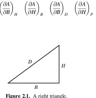
2.4. In a right triangle, such as that illustrated in Figure 2.1, the following relation-ships are valid:

D2 ¼H2þB2 P¼HþBþD A¼(1=2)BH

a. Given the special conditions:

H¼1000 cm

compute the values of each of the following partial derivatives using conver-sion relationships if necessary:

(43)

b. Given the following different set of special conditions:

compute the values of each of the following partial derivatives using conver-sion relationships if necessary:

2.5. ConsideringUas a function of any two of the variablesP, V, andT, prove that

@U

2.6. Using the deﬁnition H¼UþPV and, when necessary, obtaining conversion

relationships by consideringH(orU) as a function of any two of the variables P,V, andT, derive the following relationships:

a. @H

2.7. By a suitable experimental arrangement, it is possible to vary the total pressureP on a pure liquid independently of variations in the vapor pressurep. (However, the temperature of both phases must be identical if they are in equilibrium.) For such a system, the dependence of the vapor pressure onPandTis given by

(44)

in whichVmlis the molar volume of liquid andDHmis the molar heat of

vapor-2.8. The lengthLof a wire is a function of the temperatureTand the tensionton the wire. The linear expansivityais deﬁned by

a¼1

and is essentially constant in a small temperature range. Likewise, the isothermal Young’s modulusYdeﬁned by

Y ¼L

in whichAis the cross-sectional area of the wire is essentially constant in a small temperature range. Prove that

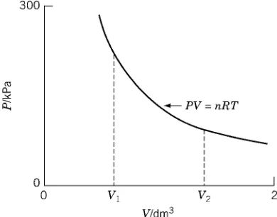
2.9. An ideal gas in State A (Fig. 2.2) is changed to State C. This transformation can be carried out by an inﬁnite number of paths. However, only two paths will be considered, one along a straight line from A to C and the other from A to B to C [9].

a. Calculate and compare the changes in volume from A to C that result from each of the two paths, AC and ABC. Proceed by integrating the differential Equation (2.2)

Before the integration is carried out along the path AC, use the following relationships to make the necessary substitutions:

slope of line AC¼T2T1 P2P1

¼TT1 PP1

(45)

Therefore

T ¼T1þ

T2T1

P2P1

(PP1) (2:48)

and

dT¼T2T1 P2P1

dP (2:49)

Remember thatT1,T2,P1, andP2are constants in this problem.

b. Applying the reciprocity test to Equation (2.6), show thatdVm is an exact

differential.

c. Calculate and compare the work performed in going from A to C by each of the two paths. Use the relationship

dW ¼ PdVm¼

RT

P dPRdT (2:50)

and the substitution suggested by Equation (2.49).

d. Applying the reciprocity test to Equation (2.50) show thatdWis not an exact differential.

2.10. For a wire, the change in lengthdLcan be expressed by the following differ-ential equation:

dL¼ L

YAdtþaLdT

in whichtis the tension andTis the temperature;A(cross-sectional area),Y, andaare essentially constant if the extension is not large (see Exercise 8).

a. IsdLan exact differential?

b. Is the differential for the work of the stretching, dW¼tdL, an exact

differential?

Figure 2.2. Two paths for carrying an ideal gas from State A to State C.

(46)

2.11. For an ideal gas we will show later that the molar entropySmis a function of the

independent variables, molar volumeVmand temperatureT. The total

differen-tialdSmis given by the equation

dSm¼(CVm=T)dTþ(R=Vm)dVm

in whichCVmandRare constants.

a. Derive an expression for the change in volume of the gas as the temperature is changed at constant entropy, that is, for (@Vm/@T)S. Your ﬁnal answer should contain only independent variables and constants.

b. IsdSmexact?

c. Derive an expression for (@CVm/@Vm)T.

2.12. The compressibilityband the coefﬁcient of expansion aare deﬁned by the partial derivatives:

2.13. For an elastic ﬁber such as a muscle ﬁbril at constant temperature, the internal energy Uis a function of three variables: the entropy S, the volume V, and the length L. With the aid of the laws of thermodynamics, it is possible to show that

dU¼TdSPdVþtdL

in whichTis the absolute temperature,Pis the pressure, andtis the tension on the elastic ﬁber. Prove the following relationships:

(47)

2.15. The Helmholtz functionAis a thermodynamic property. If (@A/@V)T¼2P

and (@A/@T)V¼2S, prove the following relationship:

@S @V

T

¼ @P

@T

V

2.16. For a van der Waals gas

dUm¼CVmdTþ

a Vm2

dVm

in whichais independent ofVm.

a. CandUmbe integrated to obtain an explicit function forUm?

b. Derive an expression for (@CVm/@Vm)T, which assumes thatdUmis exact.

2.17. Examine the following functions for homogeneity and degree of homogeneity:

a. u¼x2yþxy2þ3xyz

b. u¼x

3_þ_x2_y_þ_y3

x2_þ_xy_þ_y2

c. u¼(xþy)1=2

d. ey=x

e. u¼x

2_þ₃_xy_þ₂_y3

y2

REFERENCES

1. C. Caratheodory, Math. Ann. 67, 355 (1909); P. Frank, Thermodynamics, Brown University Press, Providence, RI, 1945; J. T. Edsall and J. Wyman, Biophysica1 Chemistry, Vol. 1, Academic Press, New York, 1958; J. G. Kirkwood and I. Oppenheim, Chemical Thermodynamics, McGraw-Hill, New York, 1961; H. A. Buchdahl, The Concepts of Classical Thermodynamics, Cambridge University Press, Cambridge, UK, 1966; O. Redlich, Rev. Mod. Phys. 40, 556 (1968); H. A. Buchdahl, Am. J. Phys.,17, 41 (1949);17, 212 (1949).

2. R. C. Tolman,Phys. Rev.9, 237 (1917).

3. P. J. Mohr and B. N. Taylor,Rev. Mod. Phys.,77, 1 – 107 (2005); http://physics.nist.gov/ constants. [R. C. Tolman,Phys. Rev.9, 237 (1917), suggested that entropy replace temp-erature in the list of base units becauseSis an extensive quantity, and all the other base quantities are extensive. Ian Mills and colleagues recommended that the kilogram be deﬁned rather than be based on a prototype mass,Metrologia,42, 71 – 80 (2005).]

(48)

4. IUPAC Compendium of Chemical Technology, 2nd ed., 1997. http://www.iupac,org/ goldbook/C00784.pdf.

5. M. A. Paul, International Union of Pure and Applied ChemistryManual of Symbols and Terminology for Physicochemical Quantities and Units, Butterworth London, 1975. 6. Quantities, Units, and Symbols, 2nd ed. A report of the Symbols Committee of the Royal

Society, London, 1975; Chemical Society Specialist Periodical Reports, Chemical ThermodynamicsVol. 1, Chap. 2, 1971; I. Mills, T. Cvitas, K. Homann, N. Kallay, and K. Kuchitsu, eds., Quantities, Units and Symbols in Physical Chemistry, 2nd ed., Blackwell Science, Oxford, UK, 1993.

7. G. Thomas, M. D. Weir, J. Hass, and F. R. GiordanoThomas’ Calculus, 11th ed., Pearson Education, Boston, 2004; J. Stewart, B. Pirtle, and K. Sandberg,Multivariate Calculus: Early Transcendentals, Brooks/Cole, Belmont, CA, 2003; R. Courant,Differential and Integral Calculus, 2nd ed., Blackie, Glasgow, Scotland, 1937.

8. For a conventional rigorous derivation in terms of limits, see H. Margenau and G. M. Murphy,The Mathematics of Physics and Chemistry, Van Nostrand, Princeton, NJ, 1st ed., 1943, pp. 6 – 8; 2nd ed., 1956, pp. 6 – 8. The approach of nonstandard analysis, however, provides a rigorous basis for the practice of treating a derivative as a ratio of inﬁnitesimals. See A. Robinson, Non-Standard Analysis, North Holland, Amsterdam, The Netherlands, 1966, pp. 79 – 83, pp. 269 – 279.

9. We have demonstrated that Equation (2.24) is a necessary condition for exactness, which is adequate for our purposes. For a proof of mathematical sufﬁciency also, see A. J. Rutgers, Physical Chemistry, Interscience, New York, 1954, p. 177, or F. T. Wall, Chemical Thermodynamics, 3rd ed., W. H. Freeman, San Francisco, CA, 1974, p. 455.

Basic Concepts and Methods

CHEMICAL

THERMODYNAMICS

Basic Concepts and Methods

CONTENTS

PREFACE

CHAPTER 1

INTRODUCTION

CHAPTER 2

MATHEMATICAL PREPARATION

FOR THERMODYNAMICS