FURTHER APPLICATIONS OF INTEGRATION

524

We looked at some applications of integrals in Chapter 6: areas, volumes, work, and average values. Here we explore some of the many other geometric applications of integration—the length of a curve, the area of a surface—as well as quantities of interest in physics, engineering, biology, economics, and statistics. For instance, we will investigate the center of gravity of a plate, the force exerted by water pressure on a dam, the flow of blood from the human heart, and the average time spent on hold during a customer support telephone call.

The length of a curve is the limit of lengths of inscribed polygons.

FURTHER

APPLICATIONS

OF INTEGRATION

What do we mean by the length of a curve? We might think of fitting a piece of string to the curve in Figure 1 and then measuring the string against a ruler. But that might be difficult to do with much accuracy if we have a complicated curve. We need a precise definition for the length of an arc of a curve, in the same spirit as the definitions we devel-oped for the concepts of area and volume.

If the curve is a polygon, we can easily find its length; we just add the lengths of the line segments that form the polygon. (We can use the distance formula to find the distance between the endpoints of each segment.) We are going to define the length of a general curve by first approximating it by a polygon and then taking a limit as the number of seg-ments of the polygon is increased. This process is familiar for the case of a circle, where the circumference is the limit of lengths of inscribed polygons (see Figure 2).

Now suppose that a curve is defined by the equation , wheref is continuous and . We obtain a polygonal approximation to by dividing the interval into nsubintervals with endpoints and equal width . If , then the point lies on and the polygon with vertices , , . . . , , illustrated in Figure 3, is an approximation to .

The length Lof is approximately the length of this polygon and the approximation gets better as we let nincrease. (See Figure 4, where the arc of the curve between and has been magnified and approximations with successively smaller values of are shown.) Therefore we define the length of the curve with equation ,

, as the limit of the lengths of these inscribed polygons (if the limit exists):

Notice that the procedure for defining arc length is very similar to the procedure we used for defining area and volume: We divided the curve into a large number of small parts. We then found the approximate lengths of the small parts and added them. Finally, we took the limit as .

The definition of arc length given by Equation 1 is not very convenient for compu-tational purposes, but we can derive an integral formula for in the case where has a continuous derivative. [Such a function is called smoothbecause a small change in produces a small change in .]

If we let , then

Pi⫺1Pi

苷sxi⫺xi⫺12⫹yi⫺yi⫺12 苷s⌬x2⫹⌬yi2

⌬yi苷yi⫺yi⫺1 f⬘x

x f

f L

n_l⬁

L_苷 lim nl⬁

n

i苷1

Pi⫺1Pi

1

a艋x艋b

y_苷fx C

L

⌬x Pi

Pi⫺1 C

F I G U R E 3

y

P¸ P¡

P™

Pi-1 _P

i Pn

y=ƒ

0 a x¡ ¤ xi-1 xi b x

C

Pn P1

P0 C

Pixi, yi

yi苷fxi ⌬x

x0, x1, . . . , xn

a, b C

a艋 x艋b

y_苷fx C

525 F I G U R E 1

Pi-1

Pi

Pi-1

Pi

Pi-1

Pi

Pi-1

Pi

F I G U R E 4 F I G U R E 2

Visual 8.1 shows an animation of Figure 2.

By applying the Mean Value Theorem to on the interval , we find that there is a number between and such that

that is, Thus we have

(since )

Therefore, by Definition 1,

We recognize this expression as being equal to

by the definition of a definite integral. This integral exists because the function is continuous. Thus we have proved the following theorem:

THE ARC LENGTH FORMULA _{If is continuous on , then the length of}

the curve , , is

If we use Leibniz notation for derivatives, we can write the arc length formula as follows:

EXAMPLE 1 _{Find the length of the arc of the semicubical parabola between the}

points and . (See Figure 5.) SOLUTION _{For the top half of the curve we have}

and so the arc length formula gives

If we substitute u_苷1⫹₄9x, then du_苷9₄dx. When x_苷1,u_苷13₄; when x_苷4,u_苷10. L_苷

y

4

1

1⫹ dy

dx

2

dx_苷

y

4

1 s1

⫹9 4xdx dy

dx 苷 3 2x12 y_苷x32

4, 8 1, 1

y2

苷x3

L_苷

y

b

a

1⫹ dy

dx

2

dx 3

L_苷

y

b as1

⫹f⬘x2 _dx a艋 x艋b

y_苷fx

a, b f⬘

2

tx苷s1⫹f⬘x2

y

b a s1

⫹f⬘x2 _dx

苷 lim

nl⬁

n

i苷1

s1⫹f⬘xi*2 ⌬x L_苷 lim

nl⬁

n

i苷1

Pi⫺1Pi

⌬x⬎0

苷s1⫹f⬘xi*2 ⌬x

苷s1⫹[f⬘xi*2 s⌬x2

苷s⌬x2⫹f⬘xi*⌬x2

Pi⫺1Pi

苷s⌬x2⫹⌬yi2

⌬yi苷f⬘xi*⌬x fxi⫺_fxi⫺1苷f⬘xi*xi⫺xi⫺1

xi xi⫺1 xi*

xi⫺1, xi f

(4, 8)

F I G U R E 5

0 x

y

(1, 1)

Therefore

M

If a curve has the equation , , and is continuous, then by inter-changing the roles of and in Formula 2 or Equation 3, we obtain the following formula for its length:

EXAMPLE 2 _{Find the length of the arc of the parabola from to .}

SOLUTION Since , we have , and Formula 4 gives

We make the trigonometric substitution , which gives and

. When , , so ; when ,

, so , say. Thus

(from Example 8 in Section 7.2)

(We could have used Formula 21 in the Table of Integrals.) Since , we have , so and

NAs a check on our answer to Example 1, notice

from Figure 5 that the arc length ought to be slightly larger than the distance from to

, which is

According to our calculation in Example 1, we have

Sure enough, this is a bit greater than the length of the line segment.

L苷271(80s10⫺13s13)7.633705

s58 7.615773

4, 8

1, 1

NFigure 6 shows the arc of the parabola whose

length is computed in Example 2, together with polygonal approximations having and

line segments, respectively. For the approximate length is , the diago-nal of a square. The table shows the approxima-tions that we get by dividing into equal subintervals. Notice that each time we double the number of sides of the polygon, we get closer to the exact length, which is

Because of the presence of the square root sign in Formulas 2 and 4, the calculation of an arc length often leads to an integral that is very difficult or even impossible to evaluate explicitly. Thus we sometimes have to be content with finding an approximation to the length of a curve, as in the following example.

EXAMPLE 3

(a) Set up an integral for the length of the arc of the hyperbola from the point to the point .

(b) Use Simpson’s Rule with to estimate the arc length. SOLUTION

(a) We have

and so the arc length is

(b) Using Simpson’s Rule (see Section 7.7) with , , , , and

, we have

M

THE ARC LENGTH FUNCTION

We will find it useful to have a function that measures the arc length of a curve from a par-ticular starting point to any other point on the curve. Thus if a smooth curve has the equation , , let be the distance along from the initial point to the point . Then is a function, called the arc length function, and, by Formula 2,

(We have replaced the variable of integration by so that does not have two meanings.) We can use Part 1 of the Fundamental Theorem of Calculus to differentiate Equation 5 (since the integrand is continuous):

ds

dx 苷s1⫹f⬘x 2

苷

1⫹

dy dx

2

6

x t

sx苷

y

x a s1

⫹f⬘t2 _dt

5

s Qx, fx P0a, fa

C sx

a艋_x艋_b y_苷fx

C 1.1321

⌬x

3 f1⫹4f1.1⫹2f1.2⫹4f1.3⫹ ⭈ ⭈ ⭈ ⫹2f1.8⫹4f1.9⫹f2 L_苷

y

2

1

1⫹ 1 x4 dx fx苷s1⫹1x4

⌬_x苷0.1 n_苷10

b_苷2 a_苷1 L_苷

y

2

1

1⫹ dy

dx

2

dx_苷

y

2

1

1⫹ 1

x4 dx苷

y

2 1

sx4⫹₁ x2 dx dy

dx 苷⫺ 1 x2 y_苷 1

x n_苷10

(

2, 12

)

1, 1

xy_苷1 V

N Checking the value of the definite integral

Equation 6 shows that the rate of change of with respect to is always at least 1 and is equal to 1 when , the slope of the curve, is 0. The differential of arc length is

and this equation is sometimes written in the symmetric form

The geometric interpretation of Equation 8 is shown in Figure 7. It can be used as a mnemonic device for remembering both of the Formulas 3 and 4. If we write , then from Equation 8 either we can solve to get (7), which gives (3), or we can solve to get

which gives (4).

EXAMPLE 4 _{Find the arc length function for the curve taking}

as the starting point.

SOLUTION _{If , then}

Thus the arc length function is given by

For instance, the arc length along the curve from to is

M

s3苷32⫹18 ln 3⫺1苷8⫹ ln 3

8 8.1373

3, f3 1, 1

苷x2⫹18 ln x⫺1

苷

y

x

1

2t⫺ 1

8t

dt苷t

2_⫹1

8 ln t

]

1

x sx苷

y

x

1 s1

⫹_f⬘_t2 _dt

s1⫹_f⬘_x2

苷2x⫹ 1 8x

苷4x2⫹ 1 2 ⫹

1

64x2 苷 2x⫹ 1 8x

2

1⫹f⬘x2

苷1⫹ 2x⫺ 1 8x

2

苷1⫹4x2⫺ 1 2 ⫹

1 64x2 f⬘_x苷2x⫺ 1

8x fx苷x2⫺18 ln x

P01, 1 y_苷x2_⫺1

8 ln x

V

ds_苷

1⫹ dx dy

2 dy

L_苷

x

ds ds2

苷dx2⫹dy2

8

ds_苷

1⫹ dy dx

2 dx 7

f⬘_x

x s

F I G U R E 7

0 x

y

dx

ds _dy

F I G U R E 9

;21– 22 _{Graph the curve and visually estimate its length. Then find}

its exact length.

21. _,

22. _,

23 – 26 _{Use Simpson’s Rule with to estimate the arc}

length of the curve. Compare your answer with the value of the integral produced by your calculator.

23. _,

1. _{Use the arc length formula (3) to find the length of the curve}

, . Check your answer by noting that the curve is a line segment and calculating its length by the distance formula.

2. _{Use the arc length formula to find the length of the curve}

, . Check your answer by noting that the curve is part of a circle.

3 – 6 _{Set up, but do not evaluate, an integral for the length of the}

curve.

3. _,

4. _,

5. _,

6.

7–18 _{Find the length of the curve.}

,

N Figure 8 shows the interpretation of the arc

length function in Example 4. Figure 9 shows the graph of this arc length function. Why is negative when is less than ?x 1

the distance traveled by the prey from the time it is dropped until the time it hits the ground. Express your answer correct to the nearest tenth of a meter.

38_{. The Gateway Arch in St. Louis (see the photo on page 256)}

was constructed using the equation

for the central curve of the arch, where and are measured in meters and . Set up an integral for the length of the arch and use your calculator to estimate the length correct to the nearest meter.

A manufacturer of corrugated metal roofing wants to produce panels that are 28 in. wide and 2 in. thick by processing flat sheets of metal as shown in the figure. The profile of the roof-ing takes the shape of a sine wave. Verify that the sine curve has equation and find the width of a flat metal sheet that is needed to make a 28-inch panel. (Use your calculator to evaluate the integral correct to four significant digits.)

40. _{(a) The figure shows a telephone wire hanging between}

two poles at and . It takes the shape of a

catenary with equation . Find the

length of the wire.

; (b) Suppose two telephone poles are 50 ft apart and the length of the wire between the poles is 51 ft. If the lowest point of the wire must be 20 ft above the ground, how high up on each pole should the wire be attached?

41. _{Find the length of the curve}

; The curves with equations , , , , . . . , are

called fat circles. Graph the curves with , , , , and to see why. Set up an integral for the length of the fat circle with . Without attempting to evaluate this inte-gral, state the value of limkl⬁L2k. y苷211.49⫺20.96 cosh 0.03291765x

;27. _{(a) Graph the curve , .}

(b) Compute the lengths of inscribed polygons with , , and sides. (Divide the interval into equal subintervals.) Illustrate by sketching these polygons (as in Figure 6). (c) Set up an integral for the length of the curve.

(d) Use your calculator to find the length of the curve to four decimal places. Compare with the approximations in part (b).

;28. _{Repeat Exercise 27 for the curve}

29. _{Use either a computer algebra system or a table of integrals to}

find the exactlength of the arc of the curve that lies

between the points and .

30. _{Use either a computer algebra system or a table of integrals to}

find the exactlength of the arc of the curve that lies between the points and . If your CAS has trouble evaluating the integral, make a substitution that changes the integral into one that the CAS can evaluate.

Sketch the curve with equation and use sym-metry to find its length.

32. _{(a) Sketch the curve .}

(b) Use Formulas 3 and 4 to set up two integrals for the arc length from to . Observe that one of these is an improper integral and evaluate both of them. (c) Find the length of the arc of this curve from

to .

Find the arc length function for the curve with starting point .

;34. _{(a) Graph the curve , .}

(b) Find the arc length function for this curve with starting point .

(c) Graph the arc length function.

35. _{Find the arc length function for the curve}

with starting point .

36. _{A steady wind blows a kite due west. The kite’s height above}

ground from horizontal position to is given

by _{. Find the distance traveled by the}

kite.

37. _{A hawk flying at at an altitude of 180 m accidentally}

drops its prey. The parabolic trajectory of the falling prey is described by the equation

until it hits the ground, where is its height above the ground and is the horizontal distance traveled in meters. Calculatex

The curves shown are all examples of graphs of continuous functions that have the following properties.

1.

2.

3. _{The area under the graph of from 0 to 1 is equal to 1.}

The lengths of these curves, however, are different.

Try to discover formulas for two functions that satisfy the given conditions 1, 2, and 3. (Your graphs might be similar to the ones shown or could look quite different.) Then calculate the arc length of each graph. The winning entry will be the one with the smallest arc length.

LÅ3.249 x y

0 1

1

LÅ2.919 x y

0 1

1

LÅ3.152 x y

0 1

1

LÅ3.213 x y

0 1

1

L

f fx艌_{0 for 0}艋_x艋₁

f0苷0 and f1苷0

f ARC LENGTH CONTEST

D I S C O V E R Y P R O J E C T

AREA OF A SURFACE OF REVOLUTION

A surface of revolution is formed when a curve is rotated about a line. Such a surface is the lateral boundary of a solid of revolution of the type discussed in Sections 6.2 and 6.3. We want to define the area of a surface of revolution in such a way that it corresponds to our intuition. If the surface area is , we can imagine that painting the surface would require the same amount of paint as does a flat region with area .

Let’s start with some simple surfaces. The lateral surface area of a circular cylinder with radius and height is taken to be because we can imagine cutting the cylin-der and unrolling it (as in Figure 1) to obtain a rectangle with dimensions and .

Likewise, we can take a circular cone with base radius and slant height , cut it along the dashed line in Figure 2, and flatten it to form a sector of a circle with radius and cen-tral angle . We know that, in general, the area of a sector of a circle with radius

and angle is (see Exercise 35 in Section 7.3) and so in this case the area is

Therefore we define the lateral surface area of a cone to be A_苷␲_rl. A苷12l2␪苷

1 2l2

2␲_r

l

苷␲rl 1

2l2␪

␪ l

␪_苷2␲_rl

l l r

h 2␲_r A_苷2␲_rh

h r

A A

8.2

h

2πr

F I G U R E 1

What about more complicated surfaces of revolution? If we follow the strategy we used with arc length, we can approximate the original curve by a polygon. When this polygon is rotated about an axis, it creates a simpler surface whose surface area approximates the actual surface area. By taking a limit, we can determine the exact surface area.

The approximating surface, then, consists of a number of bands,each formed by rotat-ing a line segment about an axis. To find the surface area, each of these bands can be considered a portion of a circular cone, as shown in Figure 3. The area of the band (or frus-tum of a cone) with slant height and upper and lower radii and is found by sub-tracting the areas of two cones:

From similar triangles we have

which gives

or Putting this in Equation 1, we get

or

where is the average radius of the band.

Now we apply this formula to our strategy. Consider the surface shown in Figure 4, which is obtained by rotating the curve , , about the -axis, where is positive and has a continuous derivative. In order to define its surface area, we divide the interval into nsubintervals with endpoints and equal width , as we did in determining arc length. If , then the point lies on the curve. The part of the surface between and is approximated by taking the line segment and rotating it about the -axis. The result is a band with slant height and aver-age radius so, by Formula 2, its surface area is

2␲ yi⫺1⫹yi

2

Pi⫺1Pi

r_苷12yi⫺1⫹yi

l_苷

Pi⫺1Pi

x

Pi⫺1Pi xi

xi⫺1

Pixi, yi yi苷fxi

⌬_x x0, x1, . . . , xn

a, b

f x

a艋 _x艋_b y_苷fx

r_苷12r1⫹r2

A_苷2␲_rl 2

A_苷␲_r1l⫹r2l

r2⫺r1l1苷r1l r2l1苷r1l1⫹r1l

l1 r1 苷

l1⫹l r2

A_苷␲_r2l1⫹l⫺␲_r1l1苷␲_r2⫺r1l1⫹r2l

1

r2 r1 l

l ¨

2πr

F I G U R E 2

l

r cut

r¡

r™ l¡

l

F I G U R E 3

F I G U R E 4

0 x

y _y=ƒ

(a) Surface of revolution

P¸

P_i-1 Pi P_n yi

0 x

y

As in the proof of Theorem 8.1.2, we have

where is some number in . When is small, we have and

also , since is continuous. Therefore

and so an approximation to what we think of as the area of the complete surface of revo-lution is

This approximation appears to become better as and, recognizing (3) as a Riemann

sum for the function , we have

Therefore, in the case where is positive and has a continuous derivative, we define the

surface area of the surface obtained by rotating the curve , , about

the -axis as

With the Leibniz notation for derivatives, this formula becomes

If the curve is described as , , then the formula for surface area becomes

and both Formulas 5 and 6 can be summarized symbolically, using the notation for arc length given in Section 8.1, as

S_苷

y

2␲yds 7

S_苷

y

d

c 2␲y

冑

1⫹

冉

dx dy

冊

2 dy 6

c艋y艋d x_苷t共y兲

S_苷

y

b

a 2␲y

冑

1⫹

冉

dy dx

冊

2 dx 5

S_苷

y

b

a 2␲f共x兲s1⫹关f⬘共x兲兴

2 _dx

4 x

a艋 x艋b y_苷f共x兲

f lim

nl⬁

兺

n

i苷1

2␲f共xi*兲s1⫹关f⬘共xi*兲兴2 ⌬x_苷

y

b

a 2␲f共x兲s1⫹关f⬘共x兲兴

2 _dx

t共x兲苷2␲f共x兲s1⫹关f⬘共x兲兴2

n_l⬁

兺

n

i苷1

2␲f共xi*兲s1⫹关f⬘共xi*兲兴2 ⌬x 3

2␲ yi⫺1⫹yi

2

ⱍ

Pi⫺1Pi

ⱍ

⬇2␲f共xi*兲s1⫹关f⬘共xi*兲兴

2 _⌬x f

yi⫺1苷f共xi⫺1兲 ⬇f共xi*兲

yi_苷f共xi兲 ⬇f共xi*兲 ⌬x

关xi⫺1, xi兴 xi*

For rotation about the -axis, the surface area formula becomes

where, as before, we can use either

or

These formulas can be remembered by thinking of or as the circumference of a circle traced out by the point on the curve as it is rotated about the -axis or -axis, respectively (see Figure 5).

EXAMPLE 1 _{The curve , , is an arc of the circle .}

Find the area of the surface obtained by rotating this arc about the -axis. (The surface is a portion of a sphere of radius 2. See Figure 6.)

SOLUTION _{We have}

and so, by Formula 5, the surface area is

M

苷4␲

y

1

⫺1 1 dx苷4␲共2兲苷8␲

苷2␲

y

1

⫺1s4⫺x

2 2

s4⫺x2 dx

苷2␲

y

1

⫺1s4⫺x

2

冑

_1⫹ x

2

4⫺x2 dx S_苷

y

1

⫺1 2␲y

冑

1⫹

冉

dy dx

冊

2 dx dy

dx 苷 1

2共4⫺x2兲

⫺1兾2_共⫺2x兲

苷

⫺x

s4⫺x2 x

x2_⫹y2

苷4

⫺1艋 x艋1

y_苷s4⫺x2

V

F I G U R E 5 _{(a) Rotation about} x-axis: S=j 2πy ds (x, y)

y

circumference=2πy

x 0

y

(b) Rotation about y-axis: S=j 2πx ds (x, y) x

circumference=2πx x 0

y

y x

共x, y兲

2␲x 2␲y

ds_苷

冑

1⫹

冉

dx dy

冊

2 dy ds_苷

冑

1⫹

冉

dy

dx

冊

2

dx

S_苷

y

2␲xds 8

y

NFigure 6 shows the portion of the sphere

whose surface area is computed in Example 1.

1 x

y

EXAMPLE 2 _{The arc of the parabola from to is rotated about the}

-axis. Find the area of the resulting surface. SOLUTION 1 _Using

and

we have, from Formula 8,

Substituting , we have . Remembering to change the limits of integration, we have

EXAMPLE 3 _{Find the area of the surface generated by rotating the curve ,}

, about the -axis. SOLUTION _{Using Formula 5 with}

and dy

N Figure 7 shows the surface of revolution

whose area is computed in Example 2.

N As a check on our answer to Example 2,

notice from Figure 7 that the surface area should be close to that of a circular cylinder with the same height and radius halfway between the upper and lower radius of the surface:

. We computed that the surface area was

which seems reasonable. Alternatively, the sur-face area should be slightly larger than the area of a frustum of a cone with the same top and bottom edges. From Equation 2, this is

. 2␲共1.5兲(s10)⬇29.80

␲

6 (17s17⫺5s5)⬇30.85 2␲共1.5兲共3兲 ⬇28.27

N Another method: Use Formula 6 with

we have

(where )

(where and )

(by Example 8 in Section 7.2)

Since , we have and

17– 20 _{Use Simpson’s Rule with to approximate the area}

of the surface obtained by rotating the curve about the -axis. Compare your answer with the value of the integral produced by your calculator.

17. _, 18. _,

19. _, 20. _,

21– 22 _{Use either a CAS or a table of integrals to find the exact}

area of the surface obtained by rotating the given curve about the -axis.

21. _, 22. _,

23 – 24 _{Use a CAS to find the exact area of the surface obtained}

by rotating the curve about the -axis. If your CAS has trouble evaluating the integral, express the surface area as an integral in the other variable.

23. _, 24. _,

If the region is rotated

about the -axis, the volume of the resulting solid is finite (see Exercise 63 in Section 7.8). Show that the surface area is infinite. (The surface is shown in the figure and is known as

Gabriel’s horn.)

1– 4 _{Set up, but do not evaluate, an integral for the area of the}

surface obtained by rotating the curve about (a) the -axis and (b) the -axis.

, 2. _,

3. _, 4.

5 –12 _{Find the area of the surface obtained by rotating the curve}

about the -axis. ,

13 –16 _{The given curve is rotated about the -axis. Find the area}

of the resulting surface.

13. _,

32. _{Use the result of Exercise 31 to set up an integral to find the}

area of the surface generated by rotating the curve , , about the line . Then use a CAS to evaluate the integral.

33. _{Find the area of the surface obtained by rotating the circle}

about the line .

34. _{Show that the surface area of a zone of a sphere that lies}

between two parallel planes is , where is the diam-eter of the sphere and is the distance between the planes. (Notice that depends only on the distance between the planes and not on their location, provided that both planes intersect the sphere.)

35. _{Formula 4 is valid only when . Show that when}

is not necessarily positive, the formula for surface area becomes

36. _{Let be the length of the curve , , where}

is positive and has a continuous derivative. Let be the surface area generated by rotating the curve about the -axis. If is a positive constant, define and let be the corresponding surface area generated by the curve

,a艋x艋b. Express Stin terms of Sf and .L

-axis, find the area of the resulting surface.

27. _{(a) If , find the area of the surface generated by rotating}

the loop of the curve about the -axis. (b) Find the surface area if the loop is rotated about the

-axis.

28. _{A group of engineers is building a parabolic satellite dish}

whose shape will be formed by rotating the curve

about the -axis. If the dish is to have a 10-ft diameter and a maximum depth of 2 ft, find the value of and the surface area of the dish.

29. _{(a) The ellipse}

is rotated about the -axis to form a surface called an

ellipsoid, or prolate spheroid. Find the surface area of this ellipsoid.

(b) If the ellipse in part (a) is rotated about its minor axis (the -axis), the resulting ellipsoid is called an oblate spheroid. Find the surface area of this ellipsoid.

30. _{Find the surface area of the torus in Exercise 63 in}

Section 6.2.

If the curve , , is rotated about the horizontal line , where , find a formula for the area of the resulting surface.

f共x兲艋c

We know how to find the volume of a solid of revolution obtained by rotating a region about a horizontal or vertical line (see Section 6.2). We also know how to find the surface area of a sur-face of revolution if we rotate a curve about a horizontal or vertical line (see Section 8.2). But what if we rotate about a slanted line, that is, a line that is neither horizontal nor vertical? In this project you are asked to discover formulas for the volume of a solid of revolution and for the area of a surface of revolution when the axis of rotation is a slanted line.

Let be the arc of the curve between the points and and let

be the region bounded by , by the line (which lies entirely below ), and by the perpendiculars to the line from and .

P

ROTATING ON A SLANT

1. _{Show that the area of is}

[Hint:This formula can be verified by subtracting areas, but it will be helpful throughout the project to derive it by first approximating the area using rectangles perpendicular to the line, as shown in the figure. Use the figure to help express in terms of .]

2. _{Find the area of the region shown in the figure at the left.}

3. _{Find a formula similar to the one in Problem 1 for the volume of the solid obtained by}

rotating about the line .

4. _{Find the volume of the solid obtained by rotating the region of Problem 2 about the}

line .

5. _{Find a formula for the area of the surface obtained by rotating about the line .} 6. _{Use a computer algebra system to find the exact area of the surface obtained by rotating the}

curve , , about the line . Then approximate your result to three decimal places.

y苷12x

0艋x艋4

y苷sx

CAS

y苷mx⫹b C

y苷x⫺2

y苷mx⫹b

᏾

y=mx+b

Îu

å

tangent to C at {x_i, f(x_i)}

xi ∫ ?

Îx ?

⌬x

⌬u

1 1⫹m2

y

q

p 关f共x兲⫺mx⫺b兴关1⫹mf⬘共x兲兴dx

᏾

y

x 0

(2π, 2π)

y=x+sin x

y=x-2

APPLIC ATIONS TO PHYSICS AND ENGINEERING

Among the many applications of integral calculus to physics and engineering, we consider two here: force due to water pressure and centers of mass. As with our previous applica-tions to geometry (areas, volumes, and lengths) and to work, our strategy is to break up the physical quantity into a large number of small parts, approximate each small part, add the results, take the limit, and then evaluate the resulting integral.

HYDROSTATIC FORCE AND PRESSURE

Deep-sea divers realize that water pressure increases as they dive deeper. This is because the weight of the water above them increases.

In general, suppose that a thin horizontal plate with area square meters is submerged in a fluid of density kilograms per cubic meter at a depth meters below the surface of the fluid as in Figure 1. The fluid directly above the plate has volume , so its mass is . The force exerted by the fluid on the plate is therefore

F_苷mt_苷␳tAd m_苷␳V_苷␳Ad

V_苷Ad d

␳

A

8.3

surface of fluid

where is the acceleration due to gravity. The pressure on the plate is defined to be the force per unit area:

The SI unit for measuring pressure is newtons per square meter, which is called a pascal (abbreviation: 1 N兾m Pa). Since this is a small unit, the kilopascal (kPa) is often used. For instance, because the density of water is , the pressure at the bottom of a swimming pool 2 m deep is

An important principle of fluid pressure is the experimentally verified fact that at any point in a liquid the pressure is the same in all directions.(A diver feels the same pressure on nose and both ears.) Thus the pressure in anydirection at a depth in a fluid with mass density is given by

This helps us determine the hydrostatic force against a verticalplate or wall or dam in a fluid. This is not a straightforward problem because the pressure is not constant but increases as the depth increases.

EXAMPLE 1 _{A dam has the shape of the trapezoid shown in Figure 2. The height is}

20 m, and the width is 50 m at the top and 30 m at the bottom. Find the force on the dam due to hydrostatic pressure if the water level is 4 m from the top of the dam.

SOLUTION _{We choose a vertical -axis with origin at the surface of the water as in} Figure 3(a). The depth of the water is 16 m, so we divide the interval into sub-intervals of equal length with endpoints and we choose . The hori-zontal strip of the dam is approximated by a rectangle with height and width , where, from similar triangles in Figure 3(b),

or

and so

If is the area of the strip, then

If is small, then the pressure on the strip is almost constant and we can use Equation 1 to write

The hydrostatic force acting on the strip is the product of the pressure and the area:

Fi苷PiAi⬇1000txi*共46⫺xi*兲⌬x ith

Fi

Pi⬇1000txi* ith Pi

⌬x

Ai⬇w_i⌬x_苷共46⫺x_i*兲⌬x

ith Ai

w_i苷2共15⫹a兲_苷2

(

15⫹8⫺1₂x_i*

)

_苷46⫺x_i*

a_苷 16⫺xi*

2 苷8⫺

xi* 2 a

16⫺xi* 苷 10 20

w_i

⌬x

ith xi*僆关xi⫺1, xi兴

xi

关0, 16兴 x

V

P_苷␳td_苷␦d 1

␳

d

苷19,600 Pa 苷19.6 kPa

P_苷␳td_苷1000 kg兾m3_{⫻9.8 m兾s}2_{⫻2 m}

␳_苷1000 kg兾m3 2

苷1

P_苷 F A 苷␳td

P

t

50 m

20 m

30 m

F I G U R E 2

F I G U R E 3

(b) a

10

16-x_i* 20

(a) x 0 _4 15

15 10

Îx

N When using US Customary units, we write

, where is the weight density (as opposed to , which is the mass density). For instance, the weight density of water is ␦苷62.5 lb兾ft3.

Adding these forces and taking the limit as , we obtain the total hydrostatic force on the dam:

M

EXAMPLE 2 _{Find the hydrostatic force on one end of a cylindrical drum with radius 3 ft}

if the drum is submerged in water 10 ft deep.

SOLUTION _{In this example it is convenient to choose the axes as in Figure 4 so that the} origin is placed at the center of the drum. Then the circle has a simple equation,

. As in Example 1 we divide the circular region into horizontal strips of equal width. From the equation of the circle, we see that the length of the strip is

and so its area is

The pressure on this strip is approximately

and so the force on the strip is approximately

The total force is obtained by adding the forces on all the strips and taking the limit:

The second integral is 0 because the integrand is an odd function (see Theorem 5.5.7). The first integral can be evaluated using the trigonometric substitution , but it’s simpler to observe that it is the area of a semicircular disk with radius 3. Thus

M

苷 7875␲

2 ⬇12,370 lb F_苷875

y

3

⫺3s9⫺y 2 _dy

苷875ⴢ12␲共3兲2

y_苷3 sin ␪

苷125ⴢ7

y

3

⫺3s9⫺y

2 _dy⫺125

y

3

⫺3ys9⫺y 2 _dy

苷125

y

3

⫺3共7⫺y兲s9⫺y 2 _dy F_苷 lim

nl⬁

兺

n

i苷1

62.5共7⫺yi*兲2s9⫺共yi*兲2 ⌬y ␦diAi_苷62.5共7⫺yi*兲2s9⫺共yi*兲2 ⌬y

␦di_苷62.5共7⫺yi*兲 Ai_苷2s9⫺共yi*兲2 ⌬y 2s9⫺共yi*兲2

ith x2_⫹y2

苷9

⬇4.43⫻107 _N

苷9800

冋

23x2⫺

x3

3

册

₀

16

苷1000共9.8兲

y

16

0 共46x⫺x

2_兲dx

苷

y

16

0 1000tx共46⫺x兲dx F_苷 lim

nl⬁

兺

n

i苷1

1000txi*共46⫺xi*兲⌬x n_l⬁

F I G U R E 4

œ

œ„„„„„„„

œœ œœœœ œœ„

œ„ œ„

œœ„ œœ œœœœœœ ( œ œ œœ yi)

x xxx 0

000 y

10 10 10 10

7 7777 ddddiiii

≈

≈ ≈ ≈ ≈

≈++++¥¥¥¥¥¥=9=9=999

y yyyiiii***

Î ÎÎÎ

MOMENTS AND CENTERS OF MASS

Our main objective here is to find the point on which a thin plate of any given shape bal-ances horizontally as in Figure 5. This point is called the center of mass(or center of grav-ity) of the plate.

We first consider the simpler situation illustrated in Figure 6, where two masses and are attached to a rod of negligible mass on opposite sides of a fulcrum and at distances and from the fulcrum. The rod will balance if

This is an experimental fact discovered by Archimedes and called the Law of the Lever. (Think of a lighter person balancing a heavier one on a seesaw by sitting farther away from the center.)

Now suppose that the rod lies along the -axis with at and at and the center of mass at . If we compare Figures 6 and 7, we see that and and so Equation 2 gives

The numbers and are called the momentsof the masses and (with respect to the origin), and Equation 3 says that the center of mass is obtained by adding the moments of the masses and dividing by the total mass .

In general, if we have a system of particles with masses , . . . , located at the points , . . . , on the -axis, it can be shown similarly that the center of mass of the system is located at

where is the total mass of the system, and the sum of the individual moments

is called the moment of the system about the origin.Then Equation 4 could be rewritten as , which says that if the total mass were considered as being concentrated at the center of mass , then its moment would be the same as the moment of the system.x

mx_苷M

M_苷

兺

n

i苷1

mixi m_苷

冘

mi

x_苷

兺

n

i苷1

mixi

兺

n

i苷1

mi

苷

兺

n

i苷1

mixi

m 4

x xn

x2, x1

mn m2, m1 n

0

⁄ –x ¤

¤-x–

m¡ _–x-⁄ m™ x

F I G U R E 7

m_苷m1⫹m2 x

m2 m1 m2x2

m1x1

x_苷 m1x1⫹m2x2 m1⫹m2

3

m1x⫹m2x苷m1x1⫹m2x2 m1共x⫺x1兲苷m2共x2⫺x兲

d2苷x2⫺x d1苷x⫺x1

x

x2 m2 x1 m1 x

m1d1苷m2d2

2 d2 d1 m2

m1 P

F I G U R E 5 P

F I G U R E 6

m¡ m™

d¡

fulcrum

Now we consider a system of particles with masses , . . . , located at the points , , . . . , in the -plane as shown in Figure 8. By analogy with the one-dimensional case, we define the moment of the system about the y-axisto be

and the moment of the system about the x-axisas

Then measures the tendency of the system to rotate about the -axis and measures the tendency to rotate about the -axis.

As in the one-dimensional case, the coordinates of the center of mass are given in terms of the moments by the formulas

where is the total mass. Since and , the center of mass

is the point where a single particle of mass would have the same moments as the system.

EXAMPLE 3 _{Find the moments and center of mass of the system of objects that have}

masses 3, 4, and 8 at the points , , and , respectively. SOLUTION We use Equations 5 and 6 to compute the moments:

Since , we use Equations 7 to obtain

Thus the center of mass is . (See Figure 9.) M

Next we consider a flat plate (called a lamina) with uniform density that occupies a region of the plane. We wish to locate the center of mass of the plate, which is called the centroidof . In doing so we use the following physical principles: The symmetry principlesays that if is symmetric about a line , then the centroid of lies on . (If is reflected about , then remains the same so its centroid remains fixed. But the only fixed points lie on .) Thus the centroid of a rectangle is its center. Moments should be defined so that if the entire mass of a region is concentrated at the center of mass, then its moments remain unchanged. Also, the moment of the union of two nonoverlapping regions should be the sum of the moments of the individual regions.

l ᏾ l

᏾ l ᏾

l ᏾

᏾ ᏾

␳

(

11415, 1

)

y_苷 Mx m 苷

15 15 苷1 x_苷 My

m 苷 29 15 m_苷3⫹4⫹8_苷15

Mx苷3共1兲⫹4共⫺1兲⫹8共2兲苷15

My_苷3共⫺1兲⫹4共2兲⫹8共3兲_苷29 共3, 2兲 共2, ⫺1兲

共⫺1, 1兲 V

m 共x, y兲

my_苷Mx mx_苷My

m_苷

冘

mi

y_苷 Mx m x_苷 My

m 7

共x, y兲 x

Mx y

My

Mx苷

兺

n

i苷1

miyi 6

My苷

兺

n

i苷1

mixi 5

xy 共xn, yn兲

共x2, y2兲

共x1, y1兲

mn m2,

m1 n

m£ m¡

m™ y

0 x

‹ y£

⁄ ›

¤ fi

F I G U R E 8

F I G U R E 9 y

0 x

8

4 3

Suppose that the region is of the type shown in Figure 10(a); that is, lies between the lines and , above the -axis, and beneath the graph of , where is a continuous function. We divide the interval into n subintervals with endpoints

and equal width . We choose the sample point to be the midpoint of the th subinterval, that is, . This determines the polygonal approxima-tion to shown in Figure 10(b). The centroid of the th approximating rectangle is its center . Its area is , so its mass is

The moment of about the -axis is the product of its mass and the distance from to the -axis, which is

Adding these moments, we obtain the moment of the polygonal approximation to , and then by taking the limit as we obtain the moment of itself about the -axis:

In a similar fashion we compute the moment of about the -axis as the product of its mass and the distance from to the -axis:

Again we add these moments and take the limit to obtain the moment of about the -axis:

Just as for systems of particles, the center of mass of the plate is defined so that and . But the mass of the plate is the product of its density and its area:

and so

In summary, the center of mass of the plate (or the centroid of ) is located at the point , where

EXAMPLE 4 _{Find the center of mass of a semicircular plate of radius .}

SOLUTION In order to use (8) we place the semicircle as in Figure 11 so that

and , . Here there is no need to use the formula to calcu-late because, by the symmetry principle, the center of mass must lie on the -axis, so

. The area of the semicircle is , so

The center of mass is located at the point . M

EXAMPLE 5 _{Find the centroid of the region bounded by the curves , ,}

, and .

SOLUTION _{The area of the region is}

so Formulas 8 give

(by integration by parts)

If the region lies between two curves and , where , as illustrated in Figure 13, then the same sort of argument that led to Formulas 8 can be used to show that the centroid of is , where

(See Exercise 47.)

EXAMPLE 6 _{Find the centroid of the region bounded by the line and the}

parabola .

SOLUTION _{The region is sketched in Figure 14. We take , , , and}

in Formulas 9. First we note that the area of the region is

Therefore

The centroid is . M

We end this section by showing a surprising connection between centroids and volumes of revolution.

THEOREM OF PAPPUS _{Let be a plane region that lies entirely on one side of a} line in the plane. If is rotated about , then the volume of the resulting solid is the product of the area of and the distance traveled by the centroid of .

PROOF _{We give the proof for the special case in which the region lies between and}

as in Figure 13 and the line is the -axis. Using the method of cylindrical shells l y y_苷tx

N This theorem is named after the Greek

(see Section 6.3), we have

(by Formulas 9)

where is the distance traveled by the centroid during one rotation about the

-axis. M

EXAMPLE 7 _{A torus is formed by rotating a circle of radius about a line in the plane}

of the circle that is a distance from the center of the circle. Find the volume of the torus.

SOLUTION _{The circle has area . By the symmetry principle, its centroid is its} cen-ter and so the distance traveled by the centroid during a rotation is . Therefore, by the Theorem of Pappus, the volume of the torus is

M

The method of Example 7 should be compared with the method of Exercise 63 in Section 6.2.

V_苷Ad_苷2␲R␲r2苷2␲2r2R

d_苷2␲R A_苷␲r2

⬎r R

r V

y

d_苷2␲x

苷2␲xA苷Ad 苷2␲xA 苷2␲

y

b

a x关f共x兲⫺t共x兲兴dx V_苷

y

b

a 2␲x关f共x兲⫺t共x兲兴dx

5. 6.

8.

9. 10.

4 m

1 m 2 m

7.

6 m 6 m

1 m 1. _{An aquarium 5 ft long, 2 ft wide, and 3 ft deep is full of}

water. Find (a) the hydrostatic pressure on the bottom of the aquarium, (b) the hydrostatic force on the bottom, and (c) the hydrostatic force on one end of the aquarium.

2. _{A tank is 8 m long, 4 m wide, 2 m high, and contains kerosene}

with density to a depth of 1.5 m. Find (a) the hydro-static pressure on the bottom of the tank, (b) the hydrohydro-static force on the bottom, and (c) the hydrostatic force on one end of the tank.

3 –11 _{A vertical plate is submerged (or partially submerged) in}

water and has the indicated shape. Explain how to approximate the hydrostatic force against one side of the plate by a Riemann sum. Then express the force as an integral and evaluate it.

3. 4.

820 kg兾m3

E X E R C I S E S

19. _{A vertical, irregularly shaped plate is submerged in water.}

The table shows measurements of its width, taken at the indi-cated depths. Use Simpson’s Rule to estimate the force of the water against the plate.

20. _{(a) Use the formula of Exercise 18 to show that}

where is the -coordinate of the centroid of the plate and is its area. This equation shows that the hydrostatic force against a vertical plane region is the same as if the region were horizontal at the depth of the centroid of the region.

(b) Use the result of part (a) to give another solution to Exercise 10.

21– 22 _{Point-masses are located on the -axis as shown. Find}

the moment of the system about the origin and the center of mass .

21.

22.

23 – 24 _{The masses are located at the points . Find the}

moments and and the center of mass of the system.

23. _{, , ;}

, ,

24. _{, , , ;}

, , ,

25 – 28 _{Sketch the region bounded by the curves, and visually}

esti-mate the location of the centroid. Then find the exact coordinates of the centroid.

12. _{A large tank is designed with ends in the shape of the region}

between the curves and , measured in feet. Find the hydrostatic force on one end of the tank if it is filled to a depth of 8 ft with gasoline. (Assume the gasoline’s

den-sity is .)

A trough is filled with a liquid of density 840 kg兾m . The ends of the trough are equilateral triangles with sides 8 m long and vertex at the bottom. Find the hydrostatic force on one end of the trough.

14. _{A vertical dam has a semicircular gate as shown in the figure.}

Find the hydrostatic force against the gate.

15. _{A cube with 20-cm-long sides is sitting on the bottom of an}

aquarium in which the water is one meter deep. Estimate the hydrostatic force on (a) the top of the cube and (b) one of the sides of the cube.

16. _{A dam is inclined at an angle of from the vertical and has}

the shape of an isosceles trapezoid 100 ft wide at the top and 50 ft wide at the bottom and with a slant height of 70 ft. Find the hydrostatic force on the dam when it is full of water.

17. _{A swimming pool is 20 ft wide and 40 ft long and its bottom}

is an inclined plane, the shallow end having a depth of 3 ft and the deep end, 9 ft. If the pool is full of water, estimate the hydrostatic force on (a) the shallow end, (b) the deep end, (c) one of the sides, and (d) the bottom of the pool.

18. _{Suppose that a plate is immersed vertically in a fluid with}

density and the width of the plate is at a depth of meters beneath the surface of the fluid. If the top of the plate is at depth and the bottom is at depth , show that the hydrostatic force on one side of the plate is

40 – 41 _{Find the centroid of the region shown, not by integration,}

but by locating the centroids of the rectangles and triangles (from Exercise 39) and using additivity of moments.

40.

42. _{A rectangle with sides and is divided into two parts}

and by an arc of a parabola that has its vertex at one corner of and passes through the opposite corner. Find the centroids of both and .

43. _{If is the -coordinate of the centroid of the region that lies}

under the graph of a continuous function , where , show that

44 – 46 _{Use the Theorem of Pappus to find the volume of the}

given solid.

44. _{A sphere of radius (Use Example 4.)} 45. _{A cone with height and base radius}

46. _{The solid obtained by rotating the triangle with vertices}

, , and about the -axis

47. _{Prove Formulas 9.}

48. _{Let be the region that lies between the curves}

and , , where and are integers with

.

(a) Sketch the region .

(b) Find the coordinates of the centroid of .

(c) Try to find values of and such that the centroid lies

outside᏾.

29 –33 _{Find the centroid of the region bounded by the given}

curves.

34 –35 _{Calculate the moments and and the center of mass}

of a lamina with the given density and shape.

34. 35.

36. _{Use Simpson’s Rule to estimate the centroid of the region}

shown.

;37. _{Find the centroid of the region bounded by the curves}

and , , to three decimal places. Sketch the region and plot the centroid to see if your answer is reasonable.

;38. _{Use a graph to find approximate -coordinates of the points}

of intersection of the curves and .

Then find (approximately) the centroid of the region bounded by these curves.

39. _{Prove that the centroid of any triangle is located at the point}

APPLIC ATIONS TO ECONOMICS AND BIOLOGY

In this section we consider some applications of integration to economics (consumer sur-plus) and biology (blood flow, cardiac output). Others are described in the exercises.

CONSUMER SURPLUS

Recall from Section 4.7 that the demand function is the price that a company has to charge in order to sell units of a commodity. Usually, selling larger quantities requires lowering prices, so the demand function is a decreasing function. The graph of a typical demand function, called a demand curve, is shown in Figure 1. If is the amount of the commodity that is currently available, then is the current selling price.

We divide the interval into subintervals, each of length , and let be the right endpoint of the th subinterval, as in Figure 2. If, after the first units were sold, a total of only units had been available and the price per unit had been set at dollars, then the additional units could have been sold (but no more). The consumers who would have paid dollars placed a high value on the product; they would have paid what it was worth to them. So, in paying only dollars they have saved an amount of

savings per unitnumber of units苷关p共xi兲⫺P兴⌬x

P p共xi兲

⌬x p共xi兲

xi

xi⫺1 i

xi*苷xi

⌬x_苷X兾n n

关0, X兴

P_苷p共X兲

X x

p共x兲

8.4

0 x

p

P

X (X, P) p=p(x)

F I G U R E 1

A typical demand curve

Suppose you have a choice of two coffee cups of the type shown, one that bends outward and one inward, and you notice that they have the same height and their shapes fit together snugly. You wonder which cup holds more coffee. Of course you could fill one cup with water and pour it into the other one but, being a calculus student, you decide on a more mathematical approach. Ignoring the handles, you observe that both cups are surfaces of revolution, so you can think of the coffee as a volume of revolution.

1. _{Suppose the cups have height , cup A is formed by rotating the curve about the}

-axis, and cup B is formed by rotating the same curve about the line . Find the value of such that the two cups hold the same amount of coffee.

2. _{What does your result from Problem 1 say about the areas and shown in the figure?} 3. _{Use Pappus’s Theorem to explain your result in Problems 1 and 2.}

4. _{Based on your own measurements and observations, suggest a value for and an equation}

for x苷f共y兲and calculate the amount of coffee that each cup holds.

h A2 A1 k

x苷k y

x苷f共y兲 h

x y

0 h

k x=k

A¡

x=f(y) A™

Cup A Cup B COMPLEMENTARY COFFEE CUPS

Considering similar groups of willing consumers for each of the subintervals and adding the savings, we get the total savings:

(This sum corresponds to the area enclosed by the rectangles in Figure 2.) If we let , this Riemann sum approaches the integral

which economists call the consumer surplusfor the commodity.

The consumer surplus represents the amount of money saved by consumers in pur-chasing the commodity at price , corresponding to an amount demanded of . Figure 3 shows the interpretation of the consumer surplus as the area under the demand curve and above the line .

EXAMPLE 1 _{The demand for a product, in dollars, is}

Find the consumer surplus when the sales level is 500.

SOLUTION _{Since the number of products sold is , the corresponding price is}

Therefore, from Definition 1, the consumer surplus is

M

BLOOD FLOW

In Example 7 in Section 3.7 we discussed the law of laminar flow:

which gives the velocity of blood that flows along a blood vessel with radius and length at a distance from the central axis, where is the pressure difference between the ends of the vessel and is the viscosity of the blood. Now, in order to compute the rate of blood flow, or flux(volume per unit time), we consider smaller, equally spaced radii r1, r2,. . . .

␩

P r

l

R

v

vr_苷

P 4␩l R

2_⫺r2

苷$33,333.33

苷125500⫺0.15002⫺

0.00015003

3 苷125x⫺0.1x2⫺0.0001

冉

x3 3

冊册

₀

500

苷

y

500

0 共125⫺0.2x⫺0.0001x 2_兲dx

y

500

0 关p共x兲⫺P兴dx苷

y

500

0 共1200⫺0.2x⫺0.0001x

2_⫺1075兲dx

P_苷1200⫺共0.2兲共500兲⫺共0.0001兲共500兲2

苷1075

X_苷500 p_苷1200⫺0.2x⫺0.0001x2

V

p_苷P

X P

y

X

0 关p共x兲⫺P兴dx

1

n_l⬁

兺

n

i苷1

关p共xi兲⫺P兴⌬x

0 x

p

P

⁄ xi X

(X, P)

F I G U R E 2

0 x

p

(X, P) P

X p=p(x)

p=P consumer

surplus

The approximate area of the ring (or washer) with inner radius and outer radius is where

(See Figure 4.) If is small, then the velocity is almost constant throughout this ring and can be approximated by . Thus the volume of blood per unit time that flows across the ring is approximately

and the total volume of blood that flows across a cross-section per unit time is approxi-mately

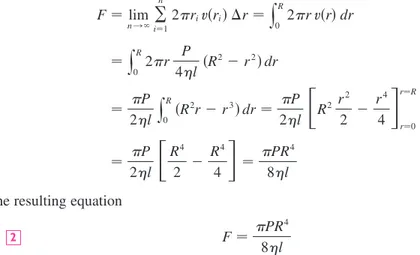
This approximation is illustrated in Figure 5. Notice that the velocity (and hence the vol-ume per unit time) increases toward the center of the blood vessel. The approximation gets better as nincreases. When we take the limit we get the exact value of the flux (or dis-charge), which is the volume of blood that passes a cross-section per unit time:

The resulting equation

is called Poiseuille’s Law; it shows that the flux is proportional to the fourth power of the radius of the blood vessel.

C ARDIAC OUTPUT

Figure 6 shows the human cardiovascular system. Blood returns from the body through the veins, enters the right atrium of the heart, and is pumped to the lungs through the pul-monary arteries for oxygenation. It then flows back into the left atrium through the pulmo-nary veins and then out to the rest of the body through the aorta. The cardiac output

of the heart is the volume of blood pumped by the heart per unit time, that is, the rate of flow into the aorta.

The dye dilution methodis used to measure the cardiac output. Dye is injected into the right atrium and flows through the heart into the aorta. A probe inserted into the aorta measures the concentration of the dye leaving the heart at equally spaced times over a time interval until the dye has cleared. Let be the concentration of the dye at time If we divide into subintervals of equal length , then the amount of dye that flows past the measuring point during the subinterval from to is approximately

concentrationvolume苷ctiF⌬t

t_苷ti t_苷ti⫺1

⌬t 关0, T兴

t. c共t兲

关0, T兴

F_苷 ␲PR 4

8␩l 2

苷

␲P 2␩l

冋

R4

2 ⫺

R4 4

册

苷

␲PR4 8␩l

苷

␲P 2␩l

y

R

0 共R

2_r⫺r3_兲dr

苷

␲P 2␩l

冋

R

2 r 2

2 ⫺

r4

4

册

_r苷0 r苷R 苷

y

R

0 2␲r P 4␩l 共R

2_⫺r2_兲dr F_苷 lim

nl⬁

兺

n

i苷1

2␲riv共ri兲⌬r_苷

y

R

0 2␲r v共r兲dr

兺

n

i苷1

2␲riv共ri兲⌬r

共2␲ri⌬r兲v共ri兲_苷2␲r_iv共ri兲⌬r v共ri兲

⌬r

⌬r_苷ri⫺ri⫺1

2␲ri⌬r

ri ri⫺1

Îr r_i

F I G U R E 4

F I G U R E 5

F I G U R E 6

aorta vein

right atrium pulmonary arteries

left atrium pulmonary veins

pulmonary veins

vein