ISTANBUL TECHNICAL UNIVERSITY INSTITUTE OF SOCIAL SCIENCES M.A. Thesis by Chynara TOLUBAEVA Department : Economics Programme : Economics June 2010
THE RELATIONSHIP BETWEEN CURRENCY CRISES AND EXCHANGE RATE REGIMES : A NON-PARAMETRIC APPROACH
ISTANBUL TECHNICAL UNIVERSITY INSTITUTE OF SOCIAL SCIENCES
THE RELATIONSHIP BETWEEN CURRENCY CRISES AND EXCHANGE RATE REGIMES : A NON-PARAMETRIC APPROACH
M.A. Thesis by Chynara TOLUBAEVA
(412081012)
Date of submission : 17 May 2010 Date of defence examination: 11 June 2010
Supervisor (Chairman) : Assist. Prof. Dr.Ahmet Atıl AŞICI (ITU) Members of the Examining Committee : Prof. Dr. Ümit ŞENESEN (ITU)
Assis. Prof. Dr. Senem ÇAKMAK ŞAHİN (YTU)
i
ISTANBUL TECHNICAL UNIVERSITY INSTITUTE OF SOCIAL SCIENCES
DÖVİZ KURU KRİZLERİ İLE DÖVİZ KURU REJİMİ ARASINDAKİ İLİŞKİLER
YÜKSEK LİSANS TEZİ Chynara TOLUBAEVA
(412081012)
Tezin Enstitüye Verildiği Tarih : 17 Mayıs 2010 Tezin Savunulduğu Tarih : 11 Haziran 2010
Tez Danışmanı : Yrd. Doç. Dr. Ahmet Atıl AŞICI (İTÜ) Diğer Jüri Üyeleri : Prof. Dr. Ümit ŞENESEN (İTÜ)
Yrd. Doç. Dr. Senem Dilek ÇAKMAK (YTÜ)
ii
FOREWORD
I would like to express my deep appreciation and thanks for my advisor and ITU Scientific Research Projects (BAP) for providing us with financial support and software facility. Furthermore, I wish to thank my parents, Jolchu Tolubaev and Inobat Tolubaeva for their love, support and understanding. So, dedicating this thesis to my parents would be the best way to express my gratidude and love for them.
June 2010 Chynara TOLUBAEVA
M.A.Economics
iii TABLE OF CONTENTS Page ABBREVIATIONS ... iv LIST OF TABLES ...v LIST OF FIGURES ... vi SUMMARY ... vii ÖZET... viii 1. INTRODUCTION ...1 2. LITERATURE REVIEW ...4
2.1 Exchange rate regime literature ... 4
2.2 Currency crises literature ... 5
2.3 The link between regime choice and currency crises ... 9
3. METHODOLOGY... 11
3.1 Advantages and disadvantages of CART ...14
3.2 Steps in CART ...16
3.3.Settings ... .17
3.3.1Types of splitting rules ... 17
3.3.2 Class assignment ... 18
3.3.3 Types of penalties ... 19
3.4 Maximal Tree construction ...20
3.5 Testing and Optimal tree selection ...20
4. EXCHANGE MARKET PRESSURE INDEX(EMPi) ... 22
5. DATA ... 26
5.1 Sample ...27
5.2 Variables of interest ...29
5.2.1.OCA Theory ... 30
5.2.2.Political view ... 30
5.2.3.Determinants of currency crises ... 31
6. CART Analysis results ... 32
6.1 Descriptive statistics ...32 6.2 Binary model ...35 6.3 Fix model ...39 6.4 Inter model ...41 6.5 Float model ...43 7. Conclusion ... 46 REFERENCES ... 48 APPENDICES ... 52
iv
ABBREVIATIONS
CC : Currency crises
ERRC : Exchange rate regime choice
LS : Levy-Yeyati and Sturzenegger
R&R : Reinhart and Rogoff
CART : Classification and Regression Trees
EMPi : Exchange Market Pressure index
OCA : Optimal currency area
EMS : European Monetary System
TN : Terminal node
v
LIST OF TABLES
Page
Table 1: LS de facto classification ... 26
Table 2: Reinhart and Rogoff de facto classification ... 28
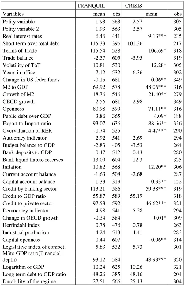
Table 3: Descriptive statistics: Tranquil vs. Crises observations ... 33
Table 4: Number of observations under Binary model ... 35
Table 5: Unconditional probabilities under Binary model ... 36
Table 6: Unconditional probabilities under Fix model ... 39
Table 7: Unconditional probabilities under Inter model ... 41
Table 8: Unconditional probabilities under Float model... 43
Table 9: Explanatory variable with references ... 52
Table 10: Variable descriptions ... 56
Table 11: List of crises cases of Binary model ... 58
Table 12: Crises observations in crisis prone TNs (Binary model) ... 60
Table 13: Terminal node information for Binary model ... 61
Table 14: Crises observations in crisis prone TNs (Fix model) ... 63
Table 15: Terminal node information for Fix model ... 64
Table 16: Crises observations in crisis prone TNs (Inter model) ... 63
Table 17: Crises observations in crisis prone TNs (Float model) ... 65
Table 18: Terminal node information for Inter model ... 66
vi
LIST OF FIGURES
Page
Figure 1 : Distributions of class A and class B. ...11
Figure 2 : The partitioning into groups. ...12
Figure 3 : Classification tree. ...13
Figure 4 : Splitting algorithm of CART ...17
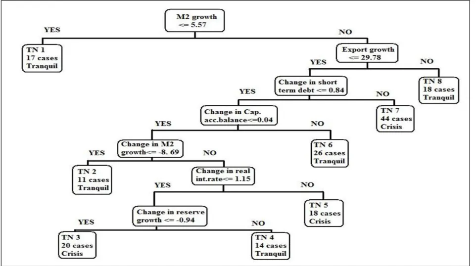
Figure 5 : Binary tree model ...37
Figure 6 : FIX tree model ...40
Figure 7 : INTER tree model ...42
vii
RELATIONSHIP BETWEEN CURRENCY CRISES AND EXCHANGE RATE REGIMES : A NON- PARAMETRIC APPROACH
SUMMARY
The crisis concept has long been an interest for economists. In this study, by using Classification and Regressin trees analysis which is a non-parametric approach, we are going to study possible relationship between regime choices and currency crises. More precisely, we are investigating whether the path leading to currency crises differs under different regimes. For instance, for a country under fixed exchange regime, the overvaluation of the real effective exchange rates could be considered as one of the causes of crises, but it is hard to find such vulnerability in a country pursuing an independently floating regime. The theoretical literature has been emphasizing the importance of regime choices, whereas it has been undervalued in empirical studies. One of our findings is that the paths leading countries to currency crises under fix, intermediate and floating regimes differ. Hence, by growing a binary classification tree for all regimes mixed in one sample, it becomes hard to detect exact relationship between crises and regime choices. Therefore, in order to get more reliable and significant results observations under each regimes should be analyzed separately. And this can be considered as the contribution of this study to the literature.
viii
DÖVİZ KURU KRİZLERİ İLE DÖVİZ KURU REJİMİ ARASINDAKİ İLİŞKİLER
ÖZET
Bu deneysel çalışmada, Sınıflandırma ve Regresyon Ağaçları (Classification and Regression trees) adlı parametrik olmayan analiz yöntemini kullanarak ülkelerin izledikleri döviz kuru rejimleri ile krize götüren sebepler arasındaki ilişkiyi araştırıyoruz. Örneğin, sabit döviz kuru rejimi altında reel döviz kuru değerlenmekte ve bu o ülkeyi krize sebep sürükleyen önemli faktörlerden biri olabilirken serbest dalgalanma rejimi altındaki bir ülkede böyle bir sorun yaşanmayabilir. Teorik kriz çalışmalarında döviz kuru önemli bir rol oynarken deneysel literatürde bu göz ardı edilmiş, örneklem seçimlerinde kur rejimine dikkat edilmemiştir. Dolayısıyla bu çalışmanın amacı birbirine doğal olarak bağlı olan ancak var olan çalışmalar tarafından işlenmemiş olan bu bağıntıyı -döviz kuru seçiminin kur krizleri ile olan ilişkisini- kurmaktır. Dalgalı, sabit ve ara kur rejimi altında olan ülkelerin kriz ve durgun gözlemlerini bir örneklem içine alarak araştırmak yanlış sonuçlar verebilir. Bu yüzden her rejime ait gözlemleri üç ayrı örneklemlere ayırarak krize uğrama yollarını araştırmak ve istatistiksel ve iktisadi anlamda daha güvenilir sonuçlara ulaştırabilir. Bu da çalışmanın literatüre yaptığı bir katkı olarak değerlendirilebilir.
1
1. INTRODUCTION
The crisis concept has long been an interest for economists. Specifically affected by the Mexican Tequila (1994), Asian flu (1997), Russian currency market instabilities in 1998 and Argentina (2001) crises, plenty of empirical researches have been done in order to identify the potential causes of speculative attacks which lead to crises. After experiencing the ―pain‖ or cost of entering the crisis period, researchers started analyzing the optimal macroeconomic policies which could prevent from entering, or at least avoid harsh economic consequences of it. Economists such as Krugman (1979) and Obstfeld (1996) have constructed so called ―generation models‖ of currency crises (CC, hereafter) in which they have been focusing on country-specific characteristics as potential causes of crises.
Contrary to Frankel (1999)1 much of policy makers have been considering an exchange rate regime choice (ERRC, hereafter) to be independent from country-specific vulnerabilities. This was the reason for peg regimes to be of high popularity among countries in post Bretton Woods‘s period, due to its beneficial effect on taming the inflation. After subsequent financial crises in Europe (1992-93), Latin America (1994-95), and Southeast Asia (1997-98), it has been acknowledged that prior models have become less helpful in explaining the causes of recent crises. Hence, the harsh experience of entering the crisis period has led to renew the models that are capable of detecting the crisis periods as well as avoiding unfavorable economic consequences of it.
Each of experienced crises episodes were of different types, which is attributable to the differentiation of the crises concept inside itself. For instance, Jacobs, Kuper and Lestano (2003) identify three types of financial crises, which are currency crises, banking and debt crises. On the other side, Kaminsky (2003) has distinguished currency crises into six varieties.
1
Frankel (1999) states that the choice of the regime should be consistent with structural (fundamental), political and financial features of the country
2
Most of empirical studies analyzed exchange rate regimes and currency crises independently from each other, mainly concentrating on the marginal contribution of various indicators and identification of currency crises periods. Compared to currency crises literature, there are limited numbers of studies which dwell on topics such as: effects of regime switching on economic growth; possibility of optimal regime etc. Being slightly differentiated in terms of methodology and data used, there are only few papers similar to ours, such as Eichengreen and Rose (1998), Haile and Pozo (2006) in which they have tested empirically the particular relevance of exchange rate regimes to currency crises. Thus, the issue of conditional probability of experiencing CC while remaining on particular regime is found in the intersection of two literatures: regime choice and currency crises.
This paper is aimed to contribute to this scarce empirical literature by assessing whether the paths leading to currency crises vary under different regimes. In addition, along with macroeconomic indicators we want to discuss the role of ERRC in making CC. In other words, we claim that inappropriately chosen regime along with country specific vulnerabilities and fragilities may lead a way to a crisis. For instance, it is reasonable to think that, a higher inflation relative to trading partners is worrisome for a fixed regime country but maybe not so much for a floating regime country since the extent of the real exchange rate overvaluation will be much higher in the former country than the latter.
In a study like this, it is important to determine which classification of exchange rate regime to choose. There are two types of classifications, known as de facto and de jure classifications. Until 2005, most of studies have been using the IMF de jure classification which includes official rates, mainly based on regimes announced by governments. However, Calvo and Reinhart (2002), Reinhart and Rogoff (2002), Obstfeld (1996) and Rogoff (1995) observed that even if some countries say that they allow to float/fix, indeed they do not- which seems to be a case of ―fear of floating/fixing‖. Furthermore, it became known that using IMF de jure classification became less reliable and yielding misleading results. For instance, R&R (2004) find that most of floating regime countries in post 80s turns out to be de facto pegs or crawling pegs. Therefore, we have been determined in using a de facto exchange rate classification. There are two types of de facto classifications, constructed by Levy-Yeyati and Sturzengger, 2005 (LS, hereafter) and Reinhart and Rogoff, 2004 (R&R,
3
hereafter), respectively. In our empirical analysis, we use a Reinhart and Rogoff exchange rate de facto classification, which is based on market-determined parallel exchange rate data. The distinguishable feature of R&R classification is that it defines broad range of exchange rate regime categories, which includes many intermediate arrangements, with different degrees of flexibility and commitment by government authorities.
In the analysis, we use a non-parametric Classification and Regression trees (CART) methodology to analyze the occurrence of currency crisis under different regimes. CART being developed by Breiman, Freidman, Stone and Olshen in 1984, has some distinguishable features over standard parametric approaches, specifically when there is a non-linear relationship rather than linear between explanatory variables, such as crises.
The remainder of this paper is organized as follows. Section 2 describes separately the brief overview of empirical and theoretical studies on currency crises and exchange rate regimes, done so far. Section 3 concentrates on methodological issues. Section 4 explains the measurement of Exchange market pressure index (EMPi). The data are described in Section 5. In section 6 we present main results of Classification and Regression Trees (CART). Finally, section 7 concludes the paper.
4
2. LITERATURE REVIEW
2.1 ERRC literature
This study aims to link two concepts, ERR choice and CC. As the financial globalization and trade linkages have been deepening in late 80s and 90s, the question of ―which regime would be appropriate for all times‖ is gaining greater importance. The theoretical literature on ERRC was initiated by Mundell (1961), in which he proposes the concept of Optimal Currency area (OCA), which explains the choice of regime to depend on country‘s structural features such as: the degree of trade integration, openness, size of the economy, and the magnitude of nominal/ real shocks the country is exposed to. Besides of OCA, countries‘ political and financial characteristics may be attributable to the regime choice. Stein and Frieden (2001), Levy-Yeyati et al. (2006) have used both political economy variables as potential determinants of regime choice.
The literature on ERRC puts forward three main concepts which may affect the choice of regimes: i) Optimal Currency area (OCA), the idea which was firstly initiated by Mundell; ii) financial view; iii) political view. In financial view, by testing the financial determinants of regime choice they analyze whether existence of currency mismatches and impossible trinity hypotheses are considered to be concerns for regime decision.
In terms of political view, authors present two arguments: ―policy crutch‖ and ―sustainability‖. They find that weak emerging economies tend to use pegged regimes as a policy anchor with the aim of taming the inflation. From the ―sustainability‖ perspective, political strength is a measure of propensity to peg. In other words, weak governments have difficulties in sustaining pegged regimes due to the deficits in domestic macroeconomic accounts.
Besides there are many other publications on potential determinants of the choice of regimes, but most of them have been investigating in parts and were not successful in a wider perspective, except for the study done by Levy-Yeyati, Sturzenneger and
5
Reggio (2006), which supports the spirit of theories mentioned in the above. Separately and jointly, authors compare how well and to what extent other approaches are successful in explaining the choice of exchange rate arrangements. A pooled logit regression for 183 countries with 1974-1999 time period was conducted, in which a dependent variable takes a value one if a country is identified as a de facto fixed regime, and is marked zero if it is classified as soft, flexible according to the Levy-Yeyati and Sturzenegger de facto exchange rate classification. They derive following conclusions: OCA theory is empirically supported in both industrial and non-industrial countries; however, the financial integration induces a more flexible regime in industrial countries, and converse holds in non-industrial economies; in terms of political view, authors come to conclusion that countries‘ choice of a peg diminishes if the government is weak and incapable to sustain it.
Another empirical analysis is conducted by Levy-Yeyati and Sturzenneger (2003) on the impact of exchange rate regimes on economic growth. Authors study how the choice of the regime affects the growth performance both in developing and industrial countries. Their data span 183 countries over the 1974-2000 periods. In their paper, they use LS exchange rate de facto classification, which differs from Reinhart and Rogoff‘s in terms explanatory variables used. To solve the problem of inconsistency between declared and actual policies, they have constructed a new classification based on Exchange rate and international reserves data for all IMF-reporting countries from 1974-2000 (2003). They find: for industrial countries regimes do not appear to have a significant role; for developing economies less flexible ERR are associated with slower growth and greater output volatility.
2.2 Currency crises literature
Due to the subsequent changes in trade and financial interdependence, the crises models have been changing. The financial crises of Latin America countries in 1960s and 1970s have led to construction of first-generation of crises models (Krugman (1979) and Flood and Garber (1984)). The main cause of first generation models is the inconsistency of expansive monetary policy and fixed exchange rate regime. In countries where capital is freely mobile, against the speculative attacks monetary authorities have two choices: either to hold a pegged regime or increase the interest rate by sustaining the floating regime. This argument is supported by so called
6
―impossible trinity‖ concept, which states that if a pegged regime country with no capital controls imposes an independent monetary policy at the same time, experiences high risk of its‘ reserve overloss. The incidence of EMS crises in early 1990s could not be explained by first generation models, which was a turning point for the development of second generation models (Morris and Shin (1995), Obtsfeld (1994 and 1996)). As main sources of fragilities it focuses on countries countercyclical policies in mature economies and self-fulfilling feature of crises. Next third generation models of crises were developed, due to the failure of existing models in explaining the causes of crises, which focuses on imperfect information and moral hazard which result in financial excess problems (Burnside, Eichenbaum and Rebelo (2004), Chang and Velasco (2001)). Further empirical studies can be listed as follows.
By analyzing the data of five currency crises episodes of previous decades, Glick and Rose (1998) could show that currency crises spread with ease across countries which are closely related to each other in terms of international trade linkages. Furthermore, they put emphasis on the fact that currency crises as well as trade linkages tend to be regional, which means that they affect countries in geographical terms. Although, according to the most known two speculative attack models presented by Krugman (1979) and Obstfeld (1996), at first sight it is hard to understand the concept of being ―regional‖ for currency crises, the authors demonstrate that trade linkages seem to be the only way for currency crises to be regional.
Eichengreen et al (1995) define an extensive definition of currency crises. It comprises a large depreciation of a currency and unsuccessful attacks which are neutralized by monetary authorities. They propose idea of an unsuccessful speculative attack which can be measured by sharp loss in international reserves and/or increase in interest rates.
In her paper, Tudela (2001) focuses on the origins of the currency crisis by using the duration analysis, in which she aims to measure the impact of different explanatory variables on countries‘ probability to leave a tranquil state- exiting to a currency crisis state. Furthermore, she tests whether the duration of time spent in a tranquil period could be a significant determinant of the likelihood of exit to a crisis period. Although most of the recent empirical studies on dating crises were of logit or probit
7
type, she uses a duration analysis as she believes that it is an innovative strategy which is able to detect the time dependency problem among indicators. According to Tudela, merely looking on currency devaluation is not a right way to forecast the crisis when the data is not limited to emerging countries, because speculative attacks on a currency can be prevented by monetary authorities, which results in unsuccessful attacks.
Similar idea was presented by Rose and Frankel (1996). The data is collected for over one hundred developing countries, starting from 1971 until 1992. Their objective was to examine the potential causes of currency crashes by relying on dataset of developing economies. According to authors, currency crash is defined as a depreciation of nominal exchange rate by at least 25 percent, and a 10 percent increase from the previous years‘ rate of nominal depreciation. The study being limited with developing countries, authors believe that it is sufficient to analyze a depreciation in nominal exchange rate as a key indicator of a currency crash, because due to the lack of data and information it is of great difficulty to measure the policy decisions for most of relevant countries.
Similar to Rose and Frankel (1996), Kumar, Moorthy and Perraudin (1998), Blanco and Garber (1986) use logit models to measure the likelihood for a country with particular economic and financial vulnerabilities to face devaluation. In contrast to Tudela‘s work, the authors focus only on emerging countries, for which the currency devaluation is considered as a warning signal of a possible currency crisis. In probabilistic estimations such as Logit/Probit, the relative importance of indicators is not emphasized.
A totally different approach was used by Kaminsky, Lizondo and Reinhart (1998), Eichengreen, Rose, and Wyplosz (1995), Kaminsky and Reinhart (1996), who examine the probability of facing a currency crisis and propose the early warning system. This system monitors the movement or behavior of several indicators prior to crisis. A currency crisis is defined to occur when an index computed by signal‘s approach, which is a weighted average of selected explanatory variables exceeds its mean by more than three standard deviations. Both mean and standard deviations are country specific, and calculated separately for countries experiencing a hyperinflation. Hence, whenever the index exceeds the threshold, the warning system
8
issues a signal, which forecasts that currency crisis may occur within the following 24 months.
There are also country specific papers written on the impact of currency crises. For instance, a case study on Indonesia was prepared by Cerra and Saxena (2000) analyses the Asian currency crises, but specifically focuses on Indonesia, because the authors argue that the clearest case of ―crisis contagion‖ issue is attributable to Indonesia. In their paper, besides of using Markov-switching models, they construct the Market Pressure Index, which is one of the measures of speculative pressure index. The main idea of the paper is that, Indonesia‘s case does not suit the first and second generation models, because prior to the crisis, most of south East Asian countries exhibited no signs of economic recession. Indeed, due to the high annual economic growth of some countries in South Asia in late 1980s and early 1990s, the title of Asian Tigers was awarded. This challenging side gave rise to new currency models which put emphasis on contagion.
Furthermore, Fratzcher (2000) points out that an importance of a contagion, which is measured by degree of real integration and financial interdependence among neighboring countries, as a macroeconomic indicator is underestimated in explaining the occurrence of crises.
Other closely related set of studies which comprises currency, banking and debt crises is named as financial crises literature. According to Bordo and Eichengreen (2000) and Bordo et al(2001) financial crises episodes include Tequila crisis which has arose due to the Mexican Peso devaluation in 1994; the Asian flu (1997) which has started right after Thailand‘s currency devaluation etc. There are plenty of different examples of financial crises resulting from different reasons; some of them were due to the currency devaluation, external debt and liabilities, or the collapse of banking sector. Hence, in both empirical and theoretical research financial crises are decomposed into three types: currency crises, banking and debt crises. Indeed, the new phenomenon named ―twin crises‖- a joint occurrence of banking and currency crises has been widespread. For instance, Glick and Hutchison (1999) analyze the scope and causes of banking and currency crises of 90 industrial and developed countries over the 1975-1997 period. They investigate the possible linkages between these two crises by using the signal-to-noise methodology. As a result of the
9
empirical investigation, they could find that financially liberalized emerging countries with high degree of openness are more prone to face the twin crises. In addition, they arrive at an opinion that occurrence of banking crises is a useful indicator of entering a currency crisis period for emerging markets. However, the converse does not hold.
The most similar work to our paper is done by Haile and Pozo (2006). They empirically test whether exchange rate regime choices affect countries entering the crisis period. Their approach differs from ours in two respects: The first is that they use extreme value theory to date the crisis episodes in contrast to our use of EMP index. And the second is that they classified regimes according to LS classification scheme where as the present paper employs RR scheme. They find that IMF de jure classification affects the likelihood of currency crises. In addition, they observe that even if actual exchange rate regime is not pegged, the announced pegged regimes increase the probability of currency crises.
2.3 The link between the regime choice and the currency crisis
The frequency of currency crisis increased significantly in the post-Bretton Woods period (Calvo and Reinhart, 2002). Some observers accuse intermediate exchange rate regimes stating that soft pegs are much more crisis prone than any other regime (Fischer 2001), whereas some of them support the view that crises could have occurred due to the inconsistency of macroeconomic policies with pegged regimes. In addition, according to McKinnon (2002) sometimes due to the moral hazard problems countries with weak banking systems are very vulnerable to speculative attacks, hence should refrain from imposing the flexible exchange rate regimes. Due to the beneficial effects on inflation, pegs regained its popularity in 80s and 90s. However, continuing currency crises which started with Mexican Peso devaluation in 1994 has left suspects on their sustainability. As a result, there has been growing interest in preference of flexible regime arrangements. Furthermore, in late 1990s empirical statistics have revealed that countries around the world are moving towards corner solutions and the ―bipolar view‖ is already taking place. Furthermore, new phenomena such as ―fear of floating‖, ―fear of pegging‖ and ―hidden pegs‖ have been widespread. According to Levy-Yeyati and Sturzenneger (2003): Fear of floating- is associated with countries that announces pegged regime although the de
10
facto exchange rate is floating; Due to the risk of speculative attacks on pegged regimes, fear of pegging- is attributable for countries which official seem to be floating, but in fact implying a stable exchange rate; Hidden pegs- correspond to countries that want to fix while keeping the door open to a limited exchange rate volatility.
Calvo and Reinhart (2002) investigate whether countries indeed move towards corner regimes as the above mentioned studies suggest by analyzing monthly data for 39 countries from January 1970 till November 1999. They specifically look at movements of nominal exchange rate, foreign reserves and interest rate and compare them across different regimes, since they conjecture that these variables would assess whether a country is moving towards a fix/floating regime. They claim that high variability in both interest rate and foreign reserves is attributable to the variation of nominal exchange rate, because governments most of the time intervene through these two monetary instruments.
11
3. METHODOLOGY
In an empirical part of this paper, I will apply a relatively new methodology – Classification and Regression Trees (CART). CART is being widely used for the last 10 years. One of the distinguished features of CART analysis is that it constructs decision trees. Being a non-parametric technique CART is able to unveil complex, nonlinear interactions of explanatory variables which is sometimes impossible to be solved by standard parametric approaches.
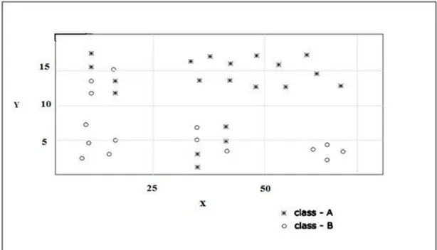
Let us explain how the classification tree analysis works by illustrating on a simple example. Assume that we have a sample of 35 observations, 20 are of class A type (crises cases) and 15 class B type (tranquil observations). For these observations, assume that we have only two indicators that seem to explain the probability of entering the crisis period (Y= short term debt to GDP ratio and X= depreciation of exchange rate). Figure 1 illustrates the scatter plot of these observations. The observations are taken as a function of X and Y, in order to ease the understanding of the incidence of crises.
12
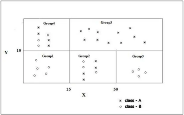
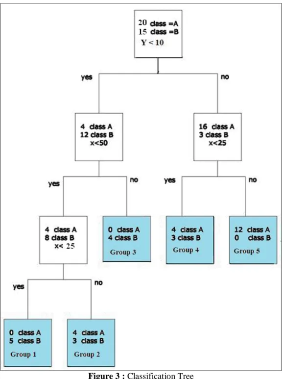
Before partitioning the sample, we need to define best splitter values for each indicator that will split observations into groups with high homogeneity. As figure 2 illustrates taking X=25, X=50 and Y=10 seem to partition observations into five distinct groups. Figure 3 illustrates the classification tree corresponding to the partitions shown in Figure2. As was early noted, the algorithm starts constructing the tree by asking ―yes/no‖ questions. For this example, the splitting started with Y<10 condition. This node is called a parent node. Due to the nature of the question posed, each parent node will have two child nodes. Observations which satisfy the Y<10 condition are separated to the left, those which do not go to right node. Left node observations are still of heterogeneous distribution, including 4 class A and 12 class B observations, hence we have to find a rule which will be able to partition further.
Figure 2 : The partitioning into groups
Observe that, for Y<10 and X>=50, we are left with no class A observations, hence X<50 is a perfect rule.
These observations form Group 3. Including the Group 3, all terminal nodes are blue colored.
Likewise, the algorithm will search for appropriate split value for each indicator, to get terminal nodes as pure as possible. As shown in the above, except for Group 2 and 4, we have isolated remaining observations perfectly. CART will not partition
13
Figure 3 : Classification Tree
observations in Group 2 and 4, because further partitioning will not increase the improvement in purity of groups. This means, further splitting will give a zero change in the degree of homogeneity of observations. Note that this is the step where algorithm stops, because splitting stops whenever there is no further improvement in purity is possible (Asici, 2010).
Once the splitting process is finished, we have to assign classes for each node. Class assignment depends on prior probabilities of each class‘ observations in a whole
14
sample. In this example, class A (class B) observations make 57% (43%) of the sample. Relying on these probabilities, a group with higher (lower) probability value than the above value will be assigned ―crisis‖ case (tranquil). As a result, due to the probability of having class A observation in Groups 2,4 and 5 is greater than 57, these terminal nodes are said to contain crisis prone observations, whereas Groups 1 and 3 tranquil.
3.1 Advantages and Disadvantages of CART
There are several advantages of CART compared over standard parametric methods. We can list them as follows:
1. CART is a non-parametric technique. This means that, there is no need to check the distribution of both dependent and independent variables used in a model. It is a time-saving feature, because a researcher is exempted from making transformation if the variables are not normally distributed.
2. CART easily deals with a problem of missing values, merely by imposing penalties on it. Hence, CART decision trees will be still generated even if the important predictor variables are not known for all observations.
3. CART is never affected by statistical model problems, such as outliers, heteroscedasticity, correlation between independent variables, autocorrelation etc. For instance, it deals with outliers by isolating them in a single node; CART solves the correlation problem by assigning closely correlated variables into the ―surrogates‖ list. So when a substantial number of observations of main predictor are missing, the algorithm allocates the best surrogates2 values instead.
4. CART results are invariant to monotone transformations of its independent variables (Timofeev 2004). In other words, if one decides to use logarithmic or squared values of an independent variable, the structure of the tree will not be changed, except for the splitting values.
2
Surrogates – are variables used as a proxy for the primary splitter. When the primary splitter value is missing, surrogate variables‘ observations replace the missing values in order to split the sample into left and right within each node. By default, CART produces five surrogates for each primary splitter at each node.
15
5. While constructing trees, CART automatically eliminates useless, insignificant indicators from being primary splitters.
On the other hand, one of the drawbacks of CART is being a non-probabilistic model. Secondly, CART‘s algorithm splits only by one variable, which means if a sample contains a complex variable capturing characteristics of one or more indicators, then CART may not perform a correct classification.
One of the applications of CART in economics is done by Asici (2010). He analyzes the power of indicators which might have a particular impact on a countries‘ decision to exit from a pegged regime to more flexible ones. In his CART model, the dependent variable is a binary EXIT, which takes a value 1 if a country exits and 0 if no exit or realignment inside the regime occurs. Furthermore, once the exit and no exit cases are identified, he classifies exit cases as orderly and disorderly exits according to the output gap variable.
Furthermore, Kaminsky (2003) uses a non- parametric method3 similar to classification trees, but not exact CART algorithm, in classifying the varieties of crises, and identifying which indicators trigger which type of crises. This new methodology partitions the data according to the characteristics of crises classes. The algorithm works as follows: at first, the observations are grouped into categories, where the tranquil and crises cases are identified. Similar to signal approach, algorithm chooses thresholds, for each indicator, which minimizes the misclassification ratio. The indicator of lowest misclassification ratio will be chosen as a first splitter. Then sample observations are divided into two subgroups: those which satisfy the threshold posed in that indicator, and which do not. For each subgroup the above procedure is repeated by assigning new threshold values for each remaining indicators. By this methodology, observations are classified into groups, of indicators satisfying the particular thresholds, each of them being identified as different types of currency crises.
The CART algorithm is not only used in economics, but it is also widely applied in many clinical research studies, household food security centers etc. For instance,
3
A methodology proposed by Kaminsky (2003), is a non-parametric alternative to the multiple-regime Markov-process models, initiated by Hamilton (1989).
16
Lewis (2000) explores CART algorithm in developing a new clinical decision rule, which is ought to be applied in various departments of Harbor-UCLA Medical center. Expected functions of clinical decision rules were: the classification of patients according to treatment or hospitalization; separate into categories of high and low risk diseases etc.
Another application of CART is the study done by Yohannes and Hoddinoff (1999). They study the indicators of Household food insecurity problem in Northern Mali. One of the distinguishing features of CART is that it selects the most relevant indicators and eliminates the least ones in explaining the dependent variable. Making use of this peculiarity, authors apply the algorithm in order to identify which indicators are most significant in providing which households result in being food insecure.
3.2 Steps in CART
According to the type of a dependent variable CART constructs either a classification or regression tree. If a dependent variable is a categorical variable, the classification tree is built, whereas for continuous dependent variable CART builds a regression tree. In our empirical analysis, we will construct three different classification trees, one for each exchange rate regimes (fix, intermediate and float), in which a categorical dependent variable takes a binary value.
After choosing options, CART starts by dividing the sample into two samples, called learning and testing samples. 90% of observations are separated for maximal tree growing; the rest 10% is left for testing the maximal tree in order to reach the optimal tree, the tree with the least misclassification cost. CART grows the biggest tree possible, called the maximal tree. In this step the aim is to reach the purest tree regardless of its representability. Although being the purest tree for the observations used, this tree may not necessarily perform the same when applied to a completely different set of observations. In CART this is done by the testing procedure. The remaining 10% of observations, called testing sample, is used to test the maximal tree. The terminal nodes which do not have the previous purity levels are pruned recursively. The pruning of the maximal tree is stopped when the misclassification cost is minimized. Hence CART algorithm involves two procedures operating exactly in the opposite direction. Maximal tree construction is defined as
purity-17
greedy segment which grows trees of highest homogeneity regardless of the node size; whereas generalization-greedy segment is defined as testing part which favours smaller trees. Once these two segments agree on a tree, the algorithm yields the optimal tree with optimal purity and generality which is later applied to new datasets. There are three main steps in CART‘s methodology: i) Choosing Option Settings (by user) ii) Construction of maximum tree (by CART methodology) iii) The testing and the choice of optimal tree (by CART methodology)
3.3 Choosing Option Settings
There are various options in CART‘s settings menu, according to which the structure of tree changes. Let‘s have a look at some of the important options, in order to have a better understanding of the way CART works.
3.3.1 Types of splitting rules
Classification trees are built according to splitting rules – rules that split learning sample into small parts. CART performs the algorithm shown in Figure 4 for each variable, where tparent is a parent node and tleft and tright are respectively left and right child nodes of a parent node, x – a variable with xR – is a best splitting value for a variable x.
Figure 4 : Splitting algorithm of CART
The important question is to determine the splitting rule which is the most appropriate and will hold for most of the observations of each significant independent variable. The key point is to isolate different types of observations into separate nodes in order to get the purest possible tree. By asking only yes or no questions the process of building a classification tree starts, splitting a whole sample in a root node to smaller and smaller parts. In each step CART searches for a best
18
split, which splits the data into two parts with maximum homogeneity. This process is continued until the maximum homogeneity in terminal nodes is attained.
There are six types of splitting rules in classification part of CART‘s theory with a specific impurity functions attached to them. We will discuss some of them briefly in here. 1) Gini splitting rule—is a most broadly used splitting criterion, which is set as a default for classification trees, puts emphasis on searching for the largest class and puts it to the right node in order to isolate it from the remaining class observations. According to Timofeev (2004) Gini is the best splitting rule for noisy data. 2) Symmetric Gini—is usually used in the case of cost matrix. 3) Entropy—is used when the target of the research is a rare class of observations. Sometimes it produces even smaller terminal nodes and compared to Gini gives less accurate classification trees. 4) Twoing—is recommended to be used when the dependent variable consists of more than two classes of observations. There are two basic differences between Gini and Twoing rule. The first one is that Twoing rule produces more balanced splits, but takes more time than Gini rule in constructing decision trees. Secondly, whenever the Twoing rule is used, the algorithm will search for two different classes, whose combination will exceed 50% of the data. Lewis (2000) suggests that Twoing and Gini give identical results if the dependent variable is a binary categorical one.
3.3.2 Class assignment
Once the maximal tree is constructed each node should be assigned a predicted class. It is necessary because if one decides to prune the sub tree or some terminal nodes, it will be impossible to know which nodes would be left as new terminal nodes. Furthermore, when the testing sample is applied to the maximal tree, the only way to be able to compute misclassification rates is to assign classes to terminal nodes in advance. The class assignment is done according to the prior probabilities of each class‘ observations in a whole sample. For instance, assume our sample consists of 100 observations, 60 are tranquil and 40 are crisis observations. Then the probability of being in tranquil (crisis) class is 60% (40%). Hence, the further class assignment of each node is done in the basis of these probabilities. Suppose if we have a terminal node whose 41% of observations are crisis dates, then we assign ―crisis class‖ to that node.
19
3.3.3 Types of penalties
In CART, at every node, every independent variable competes to become a primary splitter, but the one with high improvement score is awarded a title of a ―primary splitter‖. Sometimes, there might be a case when a primary splitting variable is missing for one or more observations. In these situations, the surrogate splitting variable‘s values replace the missing observations with primary splitter variable being kept in the sample and still preserving its title.
One may think how a variable with no missing values can be treated equally with a variable with lots of missing observations. Hence, in order to solve this problem, CART imposes penalties on variables that have got missing observations. Without penalties, it would have been unfair towards variables with no missing observations, since it is much easier for a variable to attain a higher improvement score with many missing observations. In other words, penalties lower a predictor‘s improvement score, preventing it from being chosen as a primary splitter. CART disables the penalty tab as a default option. There are three types of penalties: 1) Missing value penalties 2) High level categorical penalty 3) Predictor specific penalties
Missing value penalties are assigned both for categorical and numerical variables and may take any value between [0,2] interval. For instance, if for a variable X 30% of its observations are missing then the penalty for X should be assigned as 0.3*a, where a [0,2]. Suppose we have assigned missing value penalty equal to 2. Since the penalty rate and an improvement score are negatively correlated, by assigning 0.3, the improvement score of X will be lowered by 2*30=60%.
High level categorical penalties are imposed only on categorical variables and range between zero and five, inclusive. The concept is very much similar to that of mentioned in the above.
On the other hand, the maximum value that can predictor specific penalties be assigned is 1. Hence, observe that, by setting the penalty rate equal to 1 for a specific variable, one can totally remove that predictor from being included into the algorithm.
20
3.4 Maximal Tree Construction
Starting with a first variable, all observations of that variable founded in a parent node is split into two child nodes according to the question asked in a parent node. The question is always of the form X>t, where X is an independent variable and t is a splitting value. Observations which satisfy the condition posed in question are separated to the left child nodes and the rest goes to the right child nodes. It is very essential to divide the data into child nodes with a high homogeneity; hence the algorithm searches for the best splitting value which would maximize the homogeneity of child nodes. In CART‘s theory the maximum homogeneity in child nodes is defined by impurity function, i(t). Impurity functions are used to calculate an improvement score (the decrease in right and left child nodes). Hence, according to the impurity functions, CART repeats the above procedure for all independent variables at the root node until the maximum tree is obtained, i.e. until the sample is split up to the last observations. At the end, CART compares the splitters according to the improvement scores, and selects the variable of highest improvement score as a primary splitter. The tree building process continues until there is no any change in improvement scores of predictors, or only one observation left in each terminal node. At the end of this recursive procedure, algorithm yields us a maximal tree. In general, the maximal tree is very big in size with maximum number of terminal nodes as well as minimum degree of impurity measure. Hence, in most of cases, maximal tree is not an optimal tree, and the tree pruning option is applied to get the best final optimal tree with the least misclassification cost. In order to make more apparent explanation, let us explain how misclassification costs are computed on our model. In our sample, we have a total of 924 tranquil and 414 crisis observations. Assume the maximal tree is grown and 68 crisis observations and 27 tranquil observations have been misassigned to nodes. Hence, misclassification cost over a whole sample is found to be 0.1935, which is computed by adding two misclassification rates (68/414 + 27/924 = 0.1935)
3.5 Testing and Optimal tree Selection
As a next segment of an algorithm CART applies the testing phase. Once the maximal tree is constructed, CARTS starts pruning and we will be left with multiple of sub trees of different number of terminal nodes. In a testing procedure, the
21
performance of each sub tree is tested under different subsamples, which are generated by random sampling of the initial dataset. Usually it is very rare not to have misclassified observations in each sub tree, but the point is to select the sub tree with the least misclassification cost and the selected sub tree which will be our optimal tree.
22
4. EXCHANGE MARKET PRESSURE INDEX (EMPi)
In this section we will construct EMPi to detect crisis and tranquil dates, because in order to analyze the behaviors of crises under different regimes, we will be constructing a sample of observations consisting of crises and tranquil dates.
In currency crises literature, each of economists like Eichengreen et al. (1995, 1996), Asici et al(2007), Kaminsky, Lizondo and Reinhart (1997), Sachs, Tornell and Velasco (1996), Berg (2000) etc. have developed an index based on combination of changes in nominal exchange rates, international reserves and interest rates with purpose of detecting a speculative attack on exchange rate and forecasting CC. Although, the basic concept of this index remains same, sometimes the ―names‖ used are differentiated according to authors‘ preference. For instance, some of them prefer using Speculative pressure index (SPI), to the fact that it is widely used in capturing speculative attacks; others are in favor of using Exchange market Pressure index (EMPi), emphasizing the importance of change in exchange rates; Besides, although being rare in number, there are some economists who apply a broader version of an index and use it as an early warning system.
The motivation for constructing such index arose from the idea that speculative attacks on exchange rate regime are not always successful; hence by simply measuring the change in nominal exchange rate one is incapable of capturing all speculative pressures. Thus, it is more than important, to include all three variables stated in the above. As noted in Asici et al (2007), the inclusion of the change in interest rate is crucial and unavailability of interest rate data should not discourage you, because there are other relevant rates such as discount rate, t-bill rate and money market rates that can be used by developing countries instead of interest rates. In addition, the exclusion of interest rate sometimes gives bias results. For instance, in our sample‘s Albania February 1997 case, although the index computed by changes in exchange rate and reserves did not exceed the threshold and give a signal, the speculative pressure was detected by an increase in both t-bill and discount rates, which reveals the fact that there is no specific rule regarding which interest rate is
23
more relevant one, therefore, for each country an index should be computed by with different interest rates.
Initiated by Eichengreen et al. (1995) it has become widespread to weight the variables used in index by inverse of their standard deviation. Thus, depending on data availability and weighting preference, different versions of the following index have been used so far:
(4.1)
where the weights are taken randomly. The index has to be computed separately for countries experiencing hyperinflation; otherwise it overestimates the threshold value and gives bias values. In our study, we are going to pursue Asici et al‘s (2007) definition of hyperinflation, which is chosen to be at least 150% as an average of last 6 months.
Thus, whenever index exceeds a given threshold, which is usually taken 1.5, 2 or 3 standard deviation over its‘ mean, EMPI issues a signal. Observe that, since the value of weights taken is controversial, there is no single correct version of EMPi that could be perceived by everyone.
In this paper, we have calculated four different indices for both normal inflation and hyperinflation experiencing countries:
EMP1= (Et/ σe) – (Rt/ σr ) (4.2)
EMP3= (Et/ σe ) – (Rt/ σr ) + (Mt/ σm) (4.3)
EMP2= (Et/ σe ) – (Rt/ σr ) + (Dt/ σd) (4.4)
EMP4= (Et/ σe ) – (Rt/ σr ) + (Tt/ σt) (4.5)
where Et is the monthly depreciation of nominal exchange rates; Rt is the percentage
change in international reserves excluding gold; and Dt , Tt , Mt are monthly changes
in discount rate, t-bill rate and money market rate, respectively. For each EMP indices we have used threshold, where mean and standard deviation values are country specific. Once all four indices are computed for each country and month, we check whether
24
EMP
iµ
EMPi+ 3*σ
EMPi (4.6) for i= 1,2,3 and 4.If the (4.6) condition is satisfied, a combined index =1, otherwise it takes value 0. Furthermore, there is one more condition written below, that we have to be aware of:
EMP= 1 if none of the interest rates are available;
EMP*= max { EMP2 ,EMP3 ,EMP4 } and EMP= * if at least one of the
relevant interest rates are non-missing.
In our original dataset, at first we had 755 observations which were assigned a value of 1 for EMP. However, the total amount of EMP assembled into the sample was only 349 cases. The reason for this is that, in the procedure of detecting crises and tranquil cases, we have applied a ―three year‖ window. Starting from the first case where EMP gives a value 1, the algorithm eliminates all other possible crises dates within the time period which spans across the preceding 24 months and subsequent 12 months (t-24 to t+12). The important point is that, for an observation to be defined as crises/tranquil case, in addition to EMPi=1/0 condition we need a country to be on the same exchange rate regime for preceding 21 months. Whenever these two conditions hold, an algorithm derives the cases such as tranquil_fix / crisis_fix. For instance, if one of the observations of country A is assigned a ―crisis_fix‖ label, it should be comprehended that at that specific month, country A was using a fixed regime when it faced a speculative attack.
In previous literature, the three-year window method was used by Rose and Frankel (1996), Asici et al (2007), Eichengreen (1996), Tornell (2000) etc. Rose and Frankel (1996) applied this method while investigating the behavior of countries suffering from currency crash. They define an observation to be a currency crash, if the nominal exchange rate increases by at least 25 % and, the depreciation rate exceeds the previous year by at least 10%. They have excluded those crashes which occurred within three years from each other, in order to avoid counting the same crash twice. Asici et al(2007) conducted a research on probability of exit from pegged regimes for 128 countries. They analyze a pre-exit behavior of endogenous variables that could
25
trigger realignment within the same regime or exit to more flexible regimes, as a defending policy against speculative attacks. Similarly, for each exit and no-exit cases they have applied a three year exclusion window, to refrain from counting cases of re-pegging.
Thus, taking Asici et al (2007) work as a primary reference, for each country we will follow following steps:
- If EMPi is never equal to 1 for a country across the whole sample period, then by having the condition of ―21months being on the same regime‖ satisfied we partition the whole period as many as possible into three year subperiods. Each of these three-year subperiods will be assigned a ―tranquil‖ label.
- If a country has experienced a speculative attack only once, starting from EMPi=1 observation we apply three year window, and move up and down to assign as many as possible three year tranquil episodes.
- If a country has got more than one cases of EMPi=1, we first apply the rule in the above, then partition the time period in between of two EMPi=1 cases as to many ―tranquil‖ observations as we can.
26
5. DATA
Before detecting the crises and tranquil observations, the important thing is to decide which ERR classification is most appropriate and reliable in explaining the relationship. Levy-Yeyati and Sturzenneger (LVS) 2005; Reinhart and Rogoff (R&R) 2004 have documented that sometimes actual exchange rate regimes may differ from the announced ones, and the usage of announced regimes might lead to misleading results. As was mentioned earlier, there are two different de facto classifications: constructed by Levy-Yeyati and Sturzengger, 2005 (LS, hereafter) and Reinhart and Rogoff, 2004 (R&R, hereafter), respectively.
In LS de facto classification, exchange rate regimes are defined according to the relative behavior of three classification variables: i) Changes in nominal exchange rate ( ) ii) Volatility of percentage changes of nominal exchange rates ( ) iii) Volatility of international reserves ( );
Table 1 : LS de facto classification (2003) Classification Criteria Inconclusive low low low
Flexible high high low
Dirty float high high high Crawling peg high low high
Fixed low low high
One of their findings is that, the less flexible exchange rate regimes impel higher output volatility as well as slower growth rate in developing economies. Whereas in industrial countries, they could find no significant impact on growth. Furthermore, authors agree on the ―hollowing-out‖ effect, which is related with disappearance of soft regimes and transition to corner regimes such as currency boards, currency union, dollarization or pure floating.
In this study, we will use the de facto classification proposed by R&R, in which ERR are defined according to the behavior of ―black market‖ determined parallel
27
exchange rate data. The fine version of this classification consists of 15 exchange rate regime categories, for our study only 13 categories are used, in which corner regimes are defined as dollarization and pure floating regime. Remaining two categories are defined according to countries, for which parallel market exchange rates are missing and, experiencing a high inflation and subsequent depreciation. The latter category is called as ―freely falling‖- which highlights the fact that local currency continuingly faces a devaluation. In R&R coarse version of the classification, they arrange 13 categories into four subgroups, namely pegs, limited flexibility, managed float, and flexible regimes. The classification is described in details in Table2. To determine whether the occurrence of currency crisis under different regimes follow different paths or not, based on the announced or implicit commitment of monetary authorities, we further divide a fine classification into three subgroups, by combining the limited flexibility and managed float regimes into one category, which we will call as intermediate regimes. Hence, we are left with three broad subgroups; two of them are corner regimes- pegs and pure floating, and a soft peg- intermediate regime.
5.1 Sample
Since the updated R&R classification ends in 2007, our sample spans from 1970 till 2007. Due to the currency union dummy variable (until 2005) we have excluded countries which are in currency union area, such as countries that are included in EU etc. Hence, our initial dataset of 1338 observations has been contracted to 1030 observations. Although our crisis dating based on the index constructed by employing monthly variables, due to the lack of availability of data almost all the explanatory variables used in the analysis are annual. The detailed explanation about the explanatory variables can be found in the App. Table 9 and Table 10.
For all empirical studies, dating the incidence of crises is essential to distinguish between tranquil and crises episodes. Hence, we have defined an observation to be ―tranquil‖ period whenever there is no pressure on the currency, while a ―crisis‖ observation to be characterized by the presence of a speculative attack, either successful or not. The sampling is constructed separately for countries with hyperinflation; otherwise the magnitude of inflation overvalues the volatility of
28
Table 2 : Reinhart & Rogoff De facto regime classification
R&R categories R&R four way classificati on Three way classification
1. No separate legal tender Peg Peg
2. Pre announced peg or currency board arrangement Peg Peg 3. Pre announced horizontal band that is narrower than
or equal to +/-2% Peg Peg
4. De facto peg Peg Peg
5. Pre announced crawling peg
Limited Flexibility
Intermadiate regimes 6. Pre announced crawling band that is narrower than or
equal to +/-2%
Limited Flexibility
Intermadiate regimes 7. De factor crawling peg
Limited Flexibility
Intermadiate regimes 8. De facto crawling band that is narrower than or equal
to +/-2%
Limited Flexibility
Intermadiate regimes 9. Pre announced crawling band that is wider than or
equal to +/-2%
Limited Flexibility
Intermadiate regimes 10. De facto crawling band that is narrower than or
equal to +/-5%
Managed Float
Intermadiate regimes 11. Moving band that is narrower than or equal to
+/-2% Managed Float Intermadiate regimes 12. Managed floating Managed Float Float
13. Freely floating Pure Float Float
14. Freely falling
15. Dual market in which parallel market data is
missing
nominal exchange rates which results in using unreliable data. In order to capture both successful and unsuccessful attacks, a weighted composite of at least two variables--an Exchange Market pressure index (EMPi) is developed (Eichengreen and Rose, 1995)
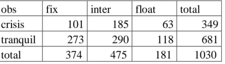
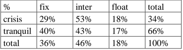
Our sample consists of 1030 observations, 681 of which are tranquil and 349 ones are crises cases. To avoid from re-counting the same crisis impact we use a three-year exclusion window around crises and tranquil dates. In total of 44 independent variables are used. The total sample includes 172 countries: 138 developing countries
29
and 34 IMF-reported advanced economies, which is based on IMF country classification. For the 1970-2007 period of time, based on observation list 46 countries have not encountered any speculative attack, and 126 countries have experienced at least one speculative attack. The complete list of crises dates for 172 countries are described in details in App. Table 11.
5.2 Variables of Interest
In an empirical part of this paper, by using information on a variety of indicators we want to analyze whether under different regime path of experiencing CC differs or not. In order to investigate the relationship between regime choice and currency crises we shall separately take a look at relevant variables that might have some effect on ERR and CC. Hence, indicators are classified into two basic groups, as determinants of ERR and CC, respectively. We have used lagged values of all indicators, as we believe the endogeneity may be concern.
One of the studies on ERR literature was done by Levy-Yeyati, Sturzenegger and Reggio (2006), in which they test three hypothesis to investigate the determinants of the regime choice question. By using a pooled logit regression for an unbalanced panel data of 183 countries, they test whether, and to what extent, the main theoretical views identified in literature are good in explaining the choice of exchange rate regimes. More precisely, they believe that there are three main approaches which are attributable for the choice of regimes: i) Theory of optimal currency area (OCA), initiated by Mundell (1961) indicates trade linkages, size, openness and the terms of trade real shocks as determinants of ERR; ii) Financial view focuses on changes that accompany financial integration and ―impossible trinity concept‖; and iii) Political economic view considers peg regimes as a ―credibility enhancers‖ for economies lacking institutional quality and political strength. In each of three approaches, authors have assembled a variety of indicators which seem to capture the closest idea highlighted in theories. Hence, by taking a de facto fixed exchange rate regime dummy as a dependent variable, they analyze to what extent the indicators are useful in determining the ERR. Let us briefly explain the main ideas of two theories of exchange rate determination.
30
5.2.1 OCA theory
According to this theory, choice of the regime is related to geographical and trade aspects of each country. This approach basically compares trade gains under pegged regimes against the benefits of more flexible regimes. In other words, OCA theory searches for macroeconomic conditions under which pegging the exchange rate is more suitable. It states that a pegged regime is desirable when there is a high degree of trade integration, and is undesirable when the economy is vulnerable to real shocks, such as terms of trade real shocks. As predicted by theory, these variables are found to affect the exchange rate regime (Klein and Marion, 1994; Edwards, 1991; Frieden et al.,2000; Levy-Yeyati et al.,2006).
Hence, theory identifies country characteristics that would like to peg or exit to a more flexible regime, such as: openness; size of the economy as proxied by log of GDP; the absence of real shocks. In order to check the validity of OCA hypothesis, we use indicators: Size- measured by taking the logarithm of GDP in current US dollar; Openness- the ratio of import plus export to GDP; and volatility of terms of trade, to measure the incidence of real shocks.
5.2.2 Political view
Various studies on exchange rate stability have focused on pegged regimes as a nominal anchor for monetary policy, specifically to tame the inflation. However, as Husain et al. (2005) finds that, there are some countries with low inflation and limited capital mobility that tend to adopt pegged regime. This is because; countries with low institutional quality are more prone on relying on fixed regime, because governments use a peg as a defending monetary instrument against the external pressures. On the other hand, Alesina (2006), Wagner (2006) has found a link between political strength and peg regimes, such that weak governments are unable to sustain pegged regimes. In our study, we use three political variables which we believe will fully reflect the political and institutional quality of countries: the number of years the incumbent administration has been in office (Years in Office); a Herfindahl index of congressional politics (Herfgov); legislative index of electoral competitiveness (Liec); Democracy indicator as a measure of institutional quality. (Levy-Yeyati,Sturzenegger and Reggio,2006) In previous empirical studies, it has been found that two of the variables (Yearsin Office and Herfindahl Index) are