How to read this book
This book may serve you better as a reference book than a textbook. It contains a large number of technical details, and we do not expect you to read it from beginning to end, since you may easily feel overwhelmed. Instead, think about your background and what you want to do first, and go to the relevant chapters or sections. For example:
I just want to finish my course homework (Chapter 2 should be more than enough for you). I know this is an R Markdown book, but I use Python more than R (Go to Section 2.7.1).
I want to embed interactive plots in my reports, or want my readers to be able change my model parameters interactively and see results on the fly (Check out Section 2.8).
I know the output format I want to use, and I want to customize its appearance (Check out the documentation of the specific output format in Chapter 3 or Chapter 4). For example, I want to customize the template for my PowerPoint presentation (Go to Section 4.4.1).
I want to build a business dashboard highlighting some key figures and indicators (Go to Chapter 5). I heard about yolo = TRUE from a friend, and I’m curious what that means in the xaringan package (Go to Chapter 7).
I want to build a personal website (Go to Chapter 10), or write a book (Go to Chapter 12). I want to write a paper and submit to the Journal of Statistical Software (Go to Chapter 13).
I want to build an interactive tutorial with exercises for my students to learn a topic (Go to Chapter 14). I’m familiar with R Markdown now, and I want to generate personalized reports for all my customers using the same R Markdown template (Try parameterized reports in Chapter 15).
I know some JavaScript, and want to build an interface in R to call an interested JavaScript library from R (Learn how to develop HTML widgets in Chapter 16).
I want to build future reports with a company branded template that shows our logo and uses our unique color theme (Go to Chapter 17).
R Markdown: The Definitive Guide
Yihui Xie, J. J. Allaire, Garrett Grolemund 2018-07-15
Preface
Note: This book is to be published by Chapman & Hall/CRC. The online version of this book is free to read here (thanks to Chapman & Hall/CRC), and licensed under the Creative Commons
Attribution-NonCommercial-ShareAlike 4.0 International License.
However, the original version of Markdown invented by John Gruber was often found overly simple and not suitable to write highly technical documents. For example, there was no syntax for tables, footnotes, math expressions, or citations. Fortunately, John MacFarlane created a wonderful package named Pandoc (http://pandoc.org) to convert Markdown documents (and many other types of documents) to a large variety of output formats. More importantly, the Markdown syntax was significantly enriched. Now we can write more types of elements with Markdown while still enjoying its simplicity.
In a nutshell, R Markdown stands on the shoulders of knitr and Pandoc. The former executes the computer code embedded in Markdown, and converts R Markdown to Markdown. The latter renders Markdown to the output format you want (such as PDF, HTML, Word, and so on).
The rmarkdown package (Allaire, Xie, McPherson, et al. 2018) was first created in early 2014. During the past four years, it has steadily evolved into a relatively complete ecosystem for authoring documents, so it is a good time for us to provide a definitive guide to this ecosystem now. At this point, there are a large number of tasks that you could do with R Markdown:
Compile a single R Markdown document to a report in different formats, such as PDF, HTML, or Word. Create notebooks in which you can directly run code chunks interactively.
Make slides for presentations (HTML5, LaTeX Beamer, or PowerPoint). Produce dashboards with flexible, interactive, and attractive layouts. Build interactive applications based on Shiny.
Write journal articles.
Author books of multiple chapters. Generate websites and blogs.
There is a fundamental assumption underneath R Markdown that users should be aware of: we assume it suffices that only a limited number of features are supported in Markdown. By “features”, we mean the types of elements you can create with native Markdown. The limitation is a great feature, not a bug. R Markdown may not be the right format for you if you find these elements not enough for your writing: paragraphs, (section) headers, block quotations, code blocks, (numbered and unnumbered) lists, horizontal rules, tables, inline formatting (emphasis, strikeout, superscripts, subscripts, verbatim, and small caps text), LaTeX math expressions, equations, links, images, footnotes, citations, theorems, proofs, and examples. We believe this list of elements suffice for most technical and non-technical documents. It may not be impossible to support other types of elements in R Markdown, but you may start to lose the simplicity of Markdown if you wish to go that far.
possible to succeed with simplicity. Jung Jae-sung was a legendary badminton player with a remarkably simple playing style: he did not look like a talented player and was very short compared to other players, so most of the time you would just see him jump three feet off the ground and smash like thunder over and over again in the back court until he beats his opponents.
Please do not underestimate the customizability of R Markdown because of the simplicity of its syntax. In particular, Pandoc templates can be surprisingly powerful, as long as you understand the underlying technologies such as LaTeX and CSS, and are willing to invest time in the appearance of your output documents (reports, books, presentations, and/or websites). As one example, you may check out the PDF report of the 2017 Employer Health Benefits Survey. It looks fairly sophisticated, but was actually
produced via bookdown (Xie 2016), which is an R Markdown extension. A custom LaTeX template and a lot of LaTeX tricks were used to generate this report. Not surprisingly, this very book that you are reading right now was also written in R Markdown, and its full source is publicly available in the GitHub repository https://github.com/rstudio/rmarkdown-book.
R Markdown documents are often portable in the sense that they can be compiled to multiple types of output formats. Again, this is mainly due to the simplified syntax of the authoring language, Markdown. The simpler the elements in your document are, the more likely that the document can be converted to different formats. Similarly, if you heavily tailor R Markdown to a specific output format (e.g., LaTeX), you are likely to lose the portability, because not all features in one format work in another format.
Last but not least, your computing results will be more likely to be reproducible if you use R Markdown (or other knitr-based source documents), compared to the manual cut-and-paste approach. This is because the results are dynamically generated from computer source code. If anything goes wrong or needs to be updated, you can simply fix or update the source code, compile the document again, and the results will automatically updated. You can enjoy reproducibility and convenience at the same time.
References
Xie, Yihui. 2015. Dynamic Documents with R and Knitr. 2nd ed. Boca Raton, Florida: Chapman; Hall/CRC. https://yihui.name/knitr/.
Xie, Yihui. 2018d. Knitr: A General-Purpose Package for Dynamic Report Generation in R. https://yihui.name/knitr/.
Structure of the book
This book consists of four parts. Part I covers the basics: Chapter 1 introduces how to install the relevant packages, and Chapter 2 is an overview of R Markdown, including the possible output formats, the Markdown syntax, the R code chunk syntax, and how to use other languages in R Markdown. Part II is the detailed documentation of built-in output formats in the rmarkdown package, including document formats and presentation formats.
Part III lists about ten R Markdown extensions that enable you to build different applications or generate output documents with different styles. Chapter 5 introduces the basics of building flexible dashboards with the R package flexdashboard. Chapter 6 documents the tufte package, which provides a unique document style used by Edward Tufte. Chapter 7 introduces the xaringan package for another highly flexible and customizable HTML5 presentation format based on the JavaScript library remark.js. Chapter 8 documents the revealjs package, which provides yet another appealing HTML5 presentation format based on the JavaScript library reveal.js. Chapter 9 introduces a few output formats created by the R community, such as the prettydoc package, which features lightweight HTML document formats. Chapter 10 teaches you how to build websites using either the blogdown package or rmarkdown’s built-in site generator. Chapter 11 explains the basics of the pkgdown package, which can be used to quickly build
documentation websites for R packages. Chapter 12 introduces how to write and publish books with the bookdown package. Chapter 13 is an overview of the rticles package for authoring journal articles. Chapter 14 introduces how to build interactive tutorials with exercises and/or quiz questions.
Part IV covers other topics about R Markdown, and some of them are advanced (in particular, Chapter 16). Chapter 15 introduces how to generate different reports with the same R Markdown source document and different parameters. Chapter 16 teaches developers how to build their own HTML widgets for interactive visualization and applications with JavaScript libraries. Chapter 17 shows how to create custom R
Markdown and Pandoc templates so that you can fully customize the appearance and style of your output document. Chapter 18 explains how to create your own output formats if the existing formats do not meet your need. Chapter 19 shows how to combine the Shiny framework with R Markdown, so that your readers can interact with the reports by changing the values of certain input widgets and seeing updated results immediately.
Software information and conventions
The R session information when compiling this book is shown below:
## R version 3.5.1 (2018-07-02)
## Platform: x86_64-apple-darwin15.6.0 (64-bit) ## Running under: macOS High Sierra 10.13.5 ##
## Locale: en_US.UTF-8 / en_US.UTF-8 / en_US.UTF-8 / C / en_US.UTF-8 / en_US.UTF-8 ## with two hashes ## by default, as you can see from the R session information above. This is for your convenience when you want to copy and run the code (the text output will be ignored since it is commented out). Package names are in bold text (e.g., rmarkdown), and inline code and filenames are formatted in a typewriter font (e.g., knitr::knit('foo.Rmd') ). Function names are followed by parentheses (e.g., blogdown::serve_site() ). The double-colon operator :: means accessing an object from a package.
“Rmd” is the filename extension of R Markdown files, and also an abbreviation of R Markdown in this book.
xfun::session_info(c(
'blogdown', 'bookdown', 'knitr', 'rmarkdown', 'htmltools', 'reticulate', 'rticles', 'flexdashboard', 'learnr', 'shiny', 'revealjs', 'pkgdown', 'tinytex', 'xaringan', 'tufte'
Acknowledgments
I started writing this book after I came back from the 2018 RStudio Conference in early February, and finished the first draft in early May. This may sound fast for a 300-page book. The main reason I was able to finish it quickly was that I worked full-time on this book for three months. My employer, RStudio, has always respected my personal interests and allowed me to focus on projects that I choose by myself. More importantly, I have been taught several lessons on how to become a professional software engineer since I joined RStudio as a fresh PhD, although the initial journey turned out to be painful. It is a great blessing for me to work in this company.
The other reason for my speed was that JJ and Garrett had already prepared a lot of materials that I could adapt for this book. They had also been offering suggestions as I worked on the manuscript. In addition, Michael Harper contributed the initial drafts of Chapters 12, 13, 15, 17, and 18. I would definitely not be able to finish this book so quickly without their help.
The most challenging thing to do when writing a book is to find large blocks of uninterrupted time. This is just so hard. Both others and myself could interrupt me. I do not consider my willpower to be strong: I read random articles, click on the endless links on Wikipedia, look at random Twitter messages, watch people fight on meaningless topics online, reply to emails all the time as if I were able to reach “Inbox Zero”, and write random blog posts from time to time. The two most important people in terms of helping keep me on track are Tareef Kawaf (President of RStudio), to whom I report my progress on the weekly basis, and Xu Qin, from whom I really learned the importance of making plans on a daily basis (although I still fail to do so sometimes). For interruptions from other people, it is impossible to isolate myself from the outside world, so I’d like to thank those who did not email me or ask me questions in the past few months and used public channels instead as I suggested. I also thank those who did not get mad at me when my responses were extremely slow or even none. I appreciate all your understanding and patience. Besides, several users have started helping me answer GitHub and Stack Overflow questions related to R
packages that I maintain, which is even better! These users include Marcel Schilling, Xianying Tan, Christophe Dervieux, and Garrick Aden-Buie, just to name a few. As someone who works from home, apparently I would not even have ten minutes of uninterrupted time if I do not send the little ones to daycare, so I want to thank all teachers at Small Miracles for freeing my daytime.
There have been a large number of contributors to the R Markdown ecosystem. More than 60 people have contributed to the core package, rmarkdown. Several authors have created their own R Markdown
extensions, as introduced in Part III of this book. Contributing ideas is no less helpful than contributing code. We have gotten numerous inspirations and ideas from the R community via various channels (GitHub issues, Stack Overflow questions, and private conversations, etc.). As a small example, Jared Lander, author of the book R for Everyone, does not meet me often, but every time he chats with me, I will get something valuable to work on. “How about writing books with R Markdown?” he asked me at the 2014 Strata conference in New York. Then we invented bookdown in 2016. “I really need fullscreen background images in ioslides. Look, Yihui, here are my ugly JavaScript hacks,” he showed me on the shuttle to dinner at the 2017 RStudio Conference. A year later, background images were officially supported in ioslides presentations.
As I was working on the draft of this book, I received a lot of helpful reviews from these reviewers: John Gillett (University of Wisconsin), Rose Hartman (UnderstandingData), Amelia McNamara (Smith College), Ariel Muldoon (Oregon State University), Yixuan Qiu (Purdue University), Benjamin Soltoff (University of Chicago), David Whitney (University of Washington), and Jon Katz (independent data analyst). Tareef Kawaf (RStudio) also volunteered to read the manuscript and provided many helpful comments. Aaron Simumba, Peter Baumgartner, and Daijiang Li volunteered to carefully correct many of my typos. In particular, Aaron has been such a big helper with my writing (not limited to only this book) and sometimes I have to compete with him in correcting my typos!
There are many colleagues at RStudio whom I want to thank for making it so convenient and even enjoyable to author R Markdown documents, especially the RStudio IDE team including J.J. Allaire, Kevin Ushey, Jonathan McPherson, and many others.
Personally I often feel motivated by members of the R community. My own willpower is weak, but I can gain a lot of power from this amazing community. Overall the community is very encouraging, and sometimes even fun, which makes me enjoy my job. For example, I do not think you can often use the picture of a professor for fun in your software, but the “desiccated baseR-er” Karl Broman is an exception (see Section 7.3.6), as he allowed me to use a mysteriously happy picture of him.
Lastly, I want to thank my editor, John Kimmel, for his continued help with my fourth book. I think I have said enough about him and his team at Chapman & Hall in my previous books. The publishing experience has always been so smooth. I just wonder if it would be possible someday that our meticulous copy-editor, Suzanne Lassandro, would fail to identify more than 30 issues for me to correct in my first draft. Probably not. Let’s see.
About the Authors
Yihui Xie
Yihui Xie (https://yihui.name) is a software engineer at RStudio (https://www.rstudio.com). He earned his PhD from the Department of Statistics, Iowa State University. He is interested in interactive statistical graphics and statistical computing. As an active R user, he has authored several R packages, such as knitr, bookdown, blogdown, xaringan, tinytex, animation, DT, tufte, formatR, fun, xfun, mime, highr, servr, and Rd2roxygen, among which the animation package won the 2009 John M. Chambers Statistical Software Award (ASA). He also co-authored a few other R packages, including shiny, rmarkdown, and leaflet.
He has authored two books, Dynamic Documents with knitr (Xie 2015), and bookdown: Authoring Books and Technical Documents with R Markdown (Xie 2016), and co-authored the book, blogdown: Creating Websites with R Markdown (Xie, Hill, and Thomas 2017).
In 2006, he founded the Capital of Statistics (https://cosx.org), which has grown into a large online
community on statistics in China. He initiated the Chinese R conference in 2008, and has been involved in organizing R conferences in China since then. During his PhD training at Iowa State University, he won the Vince Sposito Statistical Computing Award (2011) and the Snedecor Award (2012) in the Department of Statistics.
He occasionally rants on Twitter (https://twitter.com/xieyihui), and most of the time you can find him on GitHub (https://github.com/yihui).
He enjoys spicy food as much as classical Chinese literature.
References
Xie, Yihui. 2015. Dynamic Documents with R and Knitr. 2nd ed. Boca Raton, Florida: Chapman; Hall/CRC. https://yihui.name/knitr/.
Xie, Yihui. 2016. Bookdown: Authoring Books and Technical Documents with R Markdown. Boca Raton, Florida: Chapman; Hall/CRC. https://github.com/rstudio/bookdown.
J.J. Allaire
Garrett Grolemund
Chapter 1 Installation
We assume you have already installed R (https://www.r-project.org) (R Core Team 2018) and the RStudio IDE (https://www.rstudio.com). RStudio is not required but recommended, because it makes it easier for an average user to work with R Markdown. If you do not have RStudio IDE installed, you will have to install Pandoc (http://pandoc.org), otherwise there is no need to install Pandoc separately because RStudio has bundled it. Next you can install the rmarkdown package in R:
If you want to generate PDF output, you will need to install LaTeX. For R Markdown users who have not installed LaTeX before, we recommend that you install TinyTeX (https://yihui.name/tinytex/):
TinyTeX is a lightweight, portable, cross-platform, and easy-to-maintain LaTeX distribution. The R companion package tinytex (Xie 2018f) can help you automatically install missing LaTeX packages when compiling LaTeX or R Markdown documents to PDF, and also ensures a LaTeX document is compiled for the correct number of times to resolve all cross-references. If you do not understand what these two things mean, you should probably follow our recommendation to install TinyTeX, because these details are often not worth your time or attention.
With the rmarkdown package, RStudio/Pandoc, and LaTeX, you should be able to compile most R Markdown documents. In some cases, you may need other software packages, and we will mention them when necessary.
References
R Core Team. 2018. R: A Language and Environment for Statistical Computing. Vienna, Austria: R Foundation for Statistical Computing. https://www.R-project.org/.
Xie, Yihui. 2018f. Tinytex: Helper Functions to Install and Maintain Tex Live, and Compile Latex Documents. https://CRAN.R-project.org/package=tinytex.
# Install from CRAN
install.packages('rmarkdown')
# Or if you want to test the development version, # install from GitHub
if (!requireNamespace("devtools")) install.packages('devtools')
devtools::install_github('rstudio/rmarkdown')
install.packages("tinytex")
Chapter 2 Basics
R Markdown provides an authoring framework for data science. You can use a single R Markdown file to both
save and execute code, and
generate high quality reports that can be shared with an audience.
R Markdown was designed for easier reproducibility, since both the computing code and narratives are in the same document, and results are automatically generated from the source code. R Markdown supports dozens of static and dynamic/interactive output formats.
If you prefer a video introduction to R Markdown, we recommend that you check out the website
https://rmarkdown.rstudio.com, and watch the videos in the “Get Started” section, which cover the basics of R Markdown.
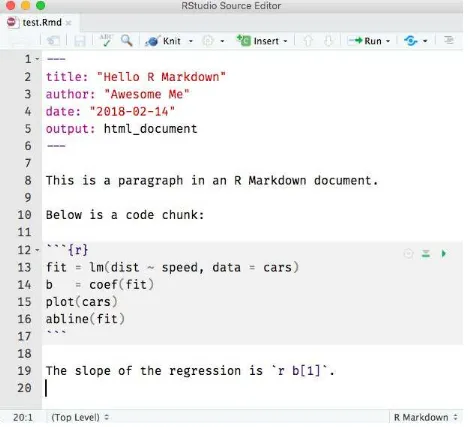
Below is a minimal R Markdown document, which should be a plain-text file, with the conventional extension .Rmd :
You can create such a text file with any editor (including but not limited to RStudio). If you use RStudio, you can create a new Rmd file from the menu File -> New File -> R Markdown .
There are three basic components of an R Markdown document: the metadata, text, and code. The metadata is written between the pair of three dashes --- . The syntax for the metadata is YAML (YAML Ain’t Markup Language, https://en.wikipedia.org/wiki/YAML), so sometimes it is also called the YAML
---title: "Hello R Markdown" author: "Awesome Me" date: "2018-02-14" output: html_document
---This is a paragraph in an R Markdown document.
Below is a code chunk:
```{r}
metadata or the YAML frontmatter. Before it bites you hard, we want to warn you in advance that indentation matters in YAML, so do not forget to indent the sub-fields of a top field properly. See the Appendix B.2 of Xie (2016) for a few simple examples that show the YAML syntax.
The body of a document follows the metadata. The syntax for text (also known as prose or narratives) is Markdown, which is introduced in Section 2.5. There are two types of computer code, which are explained in detail in Section 2.6:
A code chunk starts with three backticks like ```{r} where r indicates the language name, and ends with three backticks. You can write chunk options in the curly braces (e.g., set the figure height to 5 inches: ```{r, fig.height=5} ).
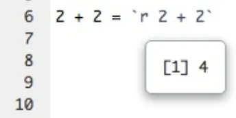
An inline R code expression starts with `r and ends with a backtick ` .
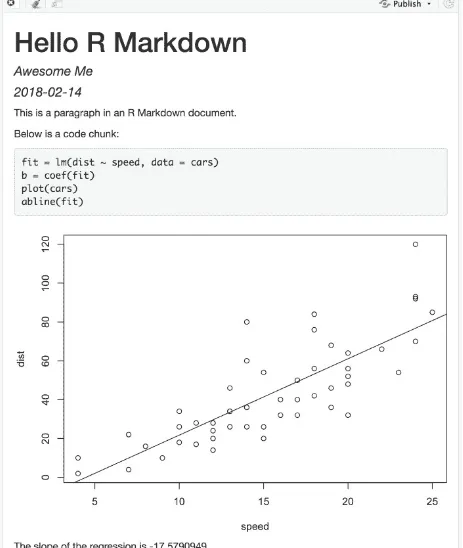
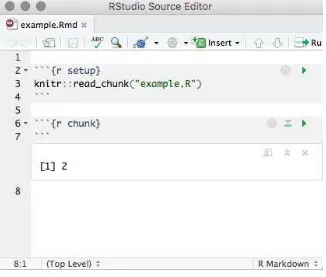
Figure 2.1 shows the above example in the RStudio IDE. You can click the Knit button to compile the document (to an HTML page). Figure 2.2 shows the output in the RStudio Viewer.
FIGURE 2.1: A minimal R Markdown example in RStudio.
FIGURE 2.2: The output document of the minimal R Markdown example in RStudio.
Now please take a closer look at the example. Did you notice a problem? The object b is the vector of coefficients of length 2 from the linear regression; b[1] is actually the intercept, and b[2] is the slope! This minimal example shows you why R Markdown is great for reproducible research: it includes the source code right inside the document, which makes it easy to discover and fix problems, as well as update the output document. All you have to do is change b[1] to b[2] , and click the Knit button again. Had you copied a number -17.579 computed elsewhere into this document, it would be very difficult to realize the problem. In fact, I had used this example a few times by myself in my presentations before I discovered this problem during one of my talks, but I discovered it anyway.
“A reproducible workflow” by Ignasi Bartomeus and Francisco Rodríguez-Sánchez
(https://youtu.be/s3JldKoA0zw). It is a 2-min video that looks artistic but also shows very common and practical problems in data analysis.
a reproducible workflow
“The Importance of Reproducible Research in High-Throughput Biology” by Keith Baggerly (https://youtu.be/7gYIs7uYbMo). You will be impressed by both the content and the style of this lecture. Keith Baggerly and Kevin Coombes were the two notable heroes in revealing the Duke/Potti scandal, which was described as “one of the biggest medical research frauds ever” by the television program “60 Minutes”.
The Importance of Reproducible Research in High-Throughput Biology
It is fine for humans to err (in computing), as long as the source code is readily available.
References
Xie, Yihui. 2016. Bookdown: Authoring Books and Technical Documents with R Markdown. Boca Raton, Florida: Chapman; Hall/CRC. https://github.com/rstudio/bookdown.
2.1 Example applications
Now you have learned the very basic concepts of R Markdown. The idea should be simple enough: interweave narratives with code in a document, knit the document to dynamically generate results from the code, and you will get a report. This idea was not invented by R Markdown, but came from an early programming paradigm called “Literate Programming” (Knuth 1984).
Due to the simplicity of Markdown and the powerful R language for data analysis, R Markdown has been widely used in many areas. Before we dive into the technical details, we want to show some examples to give you an idea of its possible applications.
2.1.1 Airbnb’s knowledge repository
Airbnb uses R Markdown to document all their analyses in R, so they can combine code and data visualizations in a single report (Bion, Chang, and Goodman 2018). Eventually all reports are carefully peer-reviewed and published to a company knowledge repository, so that anyone in the company can easily find analyses relevant to their team. Data scientists are also able to learn as much as they want from previous work or reuse the code written by previous authors, because the full R Markdown source is available in the repository.
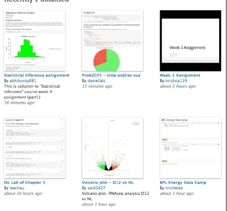
2.1.2 Homework assignments on RPubs
A huge number of homework assignments have been published to the website https://RPubs.com (a free publishing platform provided by RStudio), which shows that R Markdown is easy and convenient enough for students to do their homework assignments (see Figure 2.3). When I was still a student, I did most of my homework assignments using Sweave, which was a much earlier implementation of literate
programming based on the S language (later R) and LaTeX. I was aware of the importance of reproducible research but did not enjoy LaTeX, and few of my classmates wanted to use Sweave. Right after I
FIGURE 2.3: A screenshot of RPubs.com that contains some homework assginments submitted by students.
In a 2016 JSM (Joint Statistical Meetings) talk, I proposed that course instructors could sometimes intentionally insert some wrong values in the source data before providing it to the students for them to analyze the data in the homework, then correct these values the next time, and ask them to do the
analysis again. This way, students should be able to realize the problems with the traditional cut-and-paste approach for data analysis (i.e., run the analysis separately and copy the results manually), and the advantage of using R Markdown to automatically generate the report.
2.1.3 Personalized mail
One thing you should remember about R Markdown is that you can programmatically generate reports, although most of the time you may be just clicking the Knit button in RStudio to generate a single report from a single source document. Being able to program reports is a super power of R Markdown.
Mine Çetinkaya-Rundel once wanted to create personalized handouts for her workshop participants. She used a template R Markdown file, and knitted it in a for-loop to generate 20 PDF files for the 20
2.1.4 2017 Employer Health Benefits Survey
The 2017 Employer Health Benefits Survey was designed and analyzed by the Kaiser Family Foundation, NORC at the University of Chicago, and Health Research & Educational Trust. The full PDF report was written in R Markdown (with the bookdown package). It has a unique appearance, which was made possible by heavy customizations in the LaTeX template. This example shows you that if you really care about typesetting, you are free to apply your knowledge about LaTeX to create highly sophisticated reports from R Markdown.
2.1.5 Journal articles
Chris Hartgerink explained how and why he used R Markdown to write dynamic research documents in the post at https://elifesciences.org/labs/cad57bcf/composing-reproducible-manuscripts-using-r-markdown. He published a paper titled “Too Good to be False: Nonsignificant Results Revisited” with two co-authors (Hartgerink, Wicherts, and Assen 2017). The manuscript was written in R Markdown, and results were dynamically generated from the code in R Markdown.
When checking the accuracy of values in the psychology literature, his colleagues and he found that P-values could be mistyped or miscalculated, which could lead to inaccurate or even wrong conclusions. If the P-values were dynamically generated and inserted instead of being manually copied from statistical programs, the chance for those problems to exist would be much lower.
Lowndes et al. (2017) also shows that using R Markdown (and version control) not only enhances reproducibility, but also produces better scientific research in less time.
2.1.6 Dashboards at eelloo
R Markdown is used at eelloo (https://eelloo.nl) to design and generate research reports. Here is one of their examples (in Dutch): https://eelloo.nl/groepsrapportages-met-infographics/, where you can find gauges, bar charts, pie charts, wordclouds, and other types of graphs dynamically generated and embedded in dashboards.
2.1.7 Books
We will introduce the R Markdown extension bookdown in Chapter 12. It is an R package that allows you to write books and long-form reports with multiple Rmd files. After this package was published, a large number of books have emerged. You can find a subset of them at https://bookdown.org. Some of these books have been printed, and some only have free online versions.
There have also been students who wrote their dissertations/theses with bookdown, such as Ed Berry: https://eddjberry.netlify.com/post/writing-your-thesis-with-bookdown/. Chester Ismay has even provided an R package thesisdown (https://github.com/ismayc/thesisdown) that can render a thesis in various formats. Several other people have customized this package for their own institutions, such as Zhian N. Kamvar’s beaverdown (https://github.com/zkamvar/beaverdown) and Ben Marwick’s huskydown
(https://github.com/benmarwick/huskydown).
The blogdown package to be introduced in Chapter 10 can be used to build general-purpose websites (including blogs and personal websites) based on R Markdown. You may find tons of examples at
https://github.com/rbind or by searching on Twitter: https://twitter.com/search?q=blogdown. Here are a few impressive websites that I can quickly think of off the top of my head:
Rob J Hyndman’s personal website: https://robjhyndman.com (a very comprehensive academic website).
Amber Thomas’s personal website: https://amber.rbind.io (a rich project portfolio).
Emi Tanaka’s personal website: https://emitanaka.github.io (in particular, check out the beautiful showcase page).
“Live Free or Dichotomize” by Nick Strayer and Lucy D’Agostino McGowan:
http://livefreeordichotomize.com (the layout is elegant, and the posts are useful and practical).
References
Knuth, Donald E. 1984. “Literate Programming.” The Computer Journal 27 (2). British Computer Society: 97–111.
Bion, Ricardo, Robert Chang, and Jason Goodman. 2018. “How R Helps Airbnb Make the Most of Its Data.” The American Statistician 72 (1). Taylor & Francis: 46–52.
https://doi.org/10.1080/00031305.2017.1392362.
2.2 Compile an R Markdown document
The usual way to compile an R Markdown document is to click the Knit button as shown in Figure 2.1, and the corresponding keyboard shortcut is Ctrl + Shift + K ( Cmd + Shift + K on macOS). Under the hood, RStudio calls the function rmarkdown::render() to render the document in a new R session. Please note the emphasis here, which often confuses R Markdown users. Rendering an Rmd document in a new R session means that none of the objects in your current R session (e.g., those you created in your R console) are available to that session. Reproducibility is the main reason that RStudio uses a new R session to render your Rmd documents: in most cases, you may want your documents to continue to work the next time you open R, or in other people’s computing environments. See this StackOverflow answer if you want to know more.
If you must render a document in the current R session, you can also call rmarkdown::render() by yourself, and pass the path of the Rmd file to this function. The second argument of this function is the output format, which defaults to the first output format you specify in the YAML metadata (if it is missing, the default is html_document ). When you have multiple output formats in the metadata, and do not want to use the first one, you can specify the one you want in the second argument, e.g., for an Rmd document
foo.Rmd with the metadata:
You can render it to PDF via:
The function call gives you much more freedom (e.g., you can generate a series of reports in a loop), but you should bear reproducibility in mind when you render documents this way. Of course, you can start a new and clean R session by yourself, and call rmarkdown::render() in that session. As long as you do not manually interact with that session (e.g., manually creating variables in the R console), your reports should be reproducible.
Another main way to work with Rmd documents is the R Markdown Notebooks, which will be introduced in Section 3.2. With notebooks, you can run code chunks individually and see results right inside the RStudio editor. This is a convenient way to interact or experiment with code in an Rmd document, because you do not have to compile the whole document. Without using the notebooks, you can still partially execute code chunks, but the execution only occurs in the R console, and the notebook interface presents results of code chunks right beneath the chunks in the editor, which can be a great advantage. Again, for the sake of reproducibility, you will need to compile the whole document eventually in a clean environment.
Lastly, I want to mention an “unofficial” way to compile Rmd documents: the function
xaringan::inf_mr() , or equivalently, the RStudio addin “Infinite Moon Reader”. Obviously, this requires you to install the xaringan package (Xie 2018g), which is available on CRAN. The main advantage of this way is LiveReload: a technology that enables you to live preview the output as soon as you save the source document, and you do not need to hit the Knit button. The other advantage is that it compiles
the Rmd document in the current R session, which may or may not be what you desire. Note that this method only works for Rmd documents that output to HTML, including HTML documents and
presentations.
A few R Markdown extension packages, such as bookdown and blogdown, have their own way of compiling documents, and we will introduce them later.
Note that it is also possible to render a series of reports instead of single one from a single R Markdown source document. You can parameterize an R Markdown document, and generate different reports using different parameters. See Chapter 15 for details.
References
Xie, Yihui. 2018g. Xaringan: Presentation Ninja. https://CRAN.R-project.org/package=xaringan.
2.3 Cheat sheets
RStudio has created a large number of cheat sheets, including the one-page R Markdown cheat sheet,
which are freely available at https://www.rstudio.com/resources/cheatsheets/. There is also a more
detailed R Markdown reference guide. Both documents can be used as quick references after you become
2.4 Output formats
There are two types of output formats in the rmarkdown package: documents, and presentations. All available formats are listed below:
beamer_presentation github_document html_document
ioslides_presentation latex_document
md_document odt_document pdf_document
powerpoint_presentation rtf_document
slidy_presentation word_document
We will document these output formats in detail in Chapters 3 and 4. There are more output formats provided in other extension packages (starting from Chapter 5). For the output format names in the YAML metadata of an Rmd file, you need to include the package name if a format is from an extension package, e.g.,
If the format is from the rmarkdown package, you do not need the rmarkdown:: prefix (although it will not hurt).
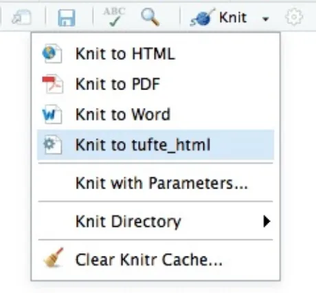
When there are multiple output formats in a document, there will be a dropdown menu behind the RStudio Knit button that lists the output format names (Figure 2.4).
FIGURE 2.4: The output formats listed in the dropdown menu on the RStudio toolbar.
Each output format is often accompanied with several format options. All these options are documented on the R package help pages. For example, you can type ?rmarkdown::html_document in R to open the help page of the html_document format. When you want to use certain options, you have to translate
the values from R to YAML, e.g.,
can be written in YAML as:
The translation is often straightforward. Remember that R’s TRUE , FALSE , and NULL are true , false , and null , respectively, in YAML. Character strings in YAML often do not require the quotes (e.g., dev: 'svg' and dev: svg are the same), unless they contain special characters, such as the colon : . If you are not sure if a string should be quoted or not, test it with the yaml package, e.g.,
Note that the subtitle in the above example is quoted because of the colon.
If a certain option has sub-options (which means the value of this option is a list in R), the sub-options need to be further indented, e.g.,
Some options are passed to knitr, such as dev , fig_width , and fig_height . Detailed documentation of these options can be found on the knitr documentation page:
https://yihui.name/knitr/options/. Note that the actual knitr option names can be different. In particular, knitr uses . in names, but rmarkdown uses _ , e.g., fig_width in rmarkdown corresponds to
fig.width in knitr. We apologize for the inconsistencies—programmers often strive for consistencies in their own world, yet one standard plus one standard often equals three standards. If I were to design the knitr package again, I would definitely use _ .
Some options are passed to Pandoc, such as toc , toc_depth , and number_sections . You should consult the Pandoc documentation when in doubt. R Markdown output format functions often have a
pandoc_args argument, which should be a character vector of extra arguments to be passed to Pandoc. html_document(toc = TRUE, toc_depth = 2, dev = 'svg')
subtitle = 'hygge: a quality of coziness' )))
title: A Wonderful Day
subtitle: 'hygge: a quality of coziness'
If you find any Pandoc features that are not represented by the output format arguments, you may use this ultimate argument, e.g.,
output:
pdf_document: toc: true
2.5 Markdown syntax
The text in an R Markdown document is written with the Markdown syntax. Precisely speaking, it is Pandoc’s Markdown. There are many flavors of Markdown invented by different people, and Pandoc’s flavor is the most comprehensive one to our knowledge. You can find the full documentation of Pandoc’s Markdown at https://pandoc.org/MANUAL.html. We strongly recommend that you read this page at least once to know all the possibilities with Pandoc’s Markdown, even if you will not use all of them. This section is adapted from Section 2.1 of Xie (2016), and only covers a small subset of Pandoc’s Markdown syntax.
2.5.1 Inline formatting
Inline text will be italic if surrounded by underscores or asterisks, e.g., _text_ or *text* . Bold text is produced using a pair of double asterisks ( **text** ). A pair of tildes ( ~ ) turn text to a subscript (e.g.,
H~3~PO~4~ renders H PO ). A pair of carets ( ^ ) produce a superscript (e.g., Cu^2+^ renders Cu ).
To mark text as inline code , use a pair of backticks, e.g., `code` . To include \(n\) literal backticks, use at least \(n+1\) backticks outside, e.g., you can use four backticks to preserve three backtick inside:
```` ```code``` ```` , which is rendered as ```code``` .
Hyperlinks are created using the syntax [text](link) , e.g., [RStudio](https://www.rstudio.com) . The syntax for images is similar: just add an exclamation mark, e.g., ![alt text or image title] (path/to/image) . Footnotes are put inside the square brackets after a caret ^[] , e.g., ^[This is a footnote.] .
There are multiple ways to insert citations, and we recommend that you use BibTeX databases, because they work better when the output format is LaTeX/PDF. Section 2.8 of Xie (2016) has explained the details. The key idea is that when you have a BibTeX database (a plain-text file with the conventional filename extension .bib ) that contains entries like:
You may add a field named bibliography to the YAML metadata, and set its value to the path of the BibTeX file. Then in Markdown, you may use @R-base (which generates “R Core Team (2018)”) or [@R-base] (which generates “(R Core Team 2018)”) to reference the BibTeX entry. Pandoc will automatically generated a list of references in the end of the document.
2.5.2 Block-level elements
Section headers can be written after a number of pound signs, e.g.,
3 4 2+
@Manual{R-base,
title = {R: A Language and Environment for Statistical Computing},
author = {{R Core Team}},
organization = {R Foundation for Statistical Computing}, address = {Vienna, Austria},
year = {2017},
If you do not want a certain heading to be numbered, you can add {-} or {.unnumbered} after the
Ordered list items start with numbers (you can also nest lists within lists), e.g.,
The output does not look too much different with the Markdown source:
1. the first item 2. the second item 3. the third item
one unordered item one unordered item
The actual output (we customized the style for blockquotes in this book):
Plain code blocks can be written after three or more backticks, and you can also indent the blocks by four spaces, e.g.,
In general, you’d better leave at least one empty line between adjacent but different elements, e.g., a header and a paragraph. This is to avoid ambiguity to the Markdown renderer. For example, does “ # ” indicate a header below?
And does “ - ” mean a bullet point below?
Different flavors of Markdown may produce different results if there are no blank lines.
2.5.3 Math expressions
Inline LaTeX equations can be written in a pair of dollar signs using the LaTeX syntax, e.g., $f(k) = {n \choose k} p^{k} (1-p)^{n-k}$ (actual output: \(f(k)={n \choose k}p^{k}(1-p)^{n-k}\)); math
expressions of the display style can be written in a pair of double dollar signs, e.g., $$f(k) = {n \choose k} p^{k} (1-p)^{n-k}$$ , and the output looks like this:
\[f\left(k\right)=\binom{n}{k}p^k\left(1-p\right)^{n-k}\]
You can also use math environments inside $ $ or $$ $$ , e.g.,
> "I thoroughly disapprove of duels. If a man should challenge me, I would take him kindly and forgivingly by the hand and lead him to a quiet place and kill him."
>
> --- Mark Twain
```
This text is displayed verbatim / preformatted ```
Or indent by four spaces:
This text is displayed verbatim / preformatted
In R, the character # indicates a comment.
\[\begin{array}{ccc} x_{11} & x_{12} & x_{13}\\ x_{21} & x_{22} & x_{23} \end{array}\]
\[X = \begin{bmatrix}1 & x_{1}\\ 1 & x_{2}\\ 1 & x_{3} \end{bmatrix}\]
\[\Theta = \begin{pmatrix}\alpha & \beta\\ \gamma & \delta \end{pmatrix}\]
\[\begin{vmatrix}a & b\\ c & d \end{vmatrix}=ad-bc\]
References
Xie, Yihui. 2016. Bookdown: Authoring Books and Technical Documents with R Markdown. Boca Raton, Florida: Chapman; Hall/CRC. https://github.com/rstudio/bookdown.
R Core Team. 2018. R: A Language and Environment for Statistical Computing. Vienna, Austria: R Foundation for Statistical Computing. https://www.R-project.org/.
$$\begin{array}{ccc} x_{11} & x_{12} & x_{13}\\ x_{21} & x_{22} & x_{23} \end{array}$$
$$X = \begin{bmatrix}1 & x_{1}\\ 1 & x_{2}\\
1 & x_{3} \end{bmatrix}$$
$$\Theta = \begin{pmatrix}\alpha & \beta\\ \gamma & \delta
\end{pmatrix}$$
$$\begin{vmatrix}a & b\\ c & d
2.6 R code chunks and inline R code
You can insert an R code chunk either using the RStudio toolbar (the Insert button) or the keyboard shortcut Ctrl + Alt + I ( Cmd + Option + I on macOS).
There are a lot of things you can do in a code chunk: you can produce text output, tables, or graphics. You have fine control over all these output via chunk options, which can be provided inside the curly braces (between ```{r and } ). For example, you can choose hide text output via the chunk option results = 'hide' , or set the figure height to 4 inches via fig.height = 4 . Chunk options are separated by commas, e.g.,
The value of a chunk option can be an arbitrary R expression, which makes chunk options extremely flexible. For example, the chunk option eval controls whether to evaluate (execute) a code chunk, and you may conditionally evaluate a chunk via a variable defined previously, e.g.,
There are a large number of chunk options in knitr documented at https://yihui.name/knitr/options. We list a subset of them below:
eval : Whether to evaluate a code chunk.
echo : Whether to echo the source code in the output document (someone may not prefer reading your smart source code but only results).
results : When set to 'hide' , text output will be hidden; when set to 'asis' , text output is written “as-is”, e.g., you can write out raw Markdown text from R code (like cat('**Markdown** is cool.\n') ). By default, text output will be wrapped in verbatim elements (typically plain code blocks).
collapse : Whether to merge text output and source code into a single code block in the output. This is mostly cosmetic: collapse = TRUE makes the output more compact, since the R source code and its text output are displayed in a single output block. The default collapse = FALSE means R expressions and their text output are separated into different blocks.
warning , message , and error : Whether to show warnings, messages, and errors in the output document. Note that if you set error = FALSE , rmarkdown::render() will halt on error in a code chunk, and the error will be displayed in the R console. Similarly, when warning = FALSE or
message = FALSE , these messages will be shown in the R console. ```{r, chunk-label, results='hide', fig.height=4}
```{r}
# execute code if the date is later than a specified day do_it = Sys.Date() > '2018-02-14'
```
include : Whether to include anything from a code chunk in the output document. When include = FALSE , this whole code chunk is excluded in the output, but note that it will still be evaluated if
eval = TRUE . When you are trying to set echo = FALSE , results = 'hide' , warning = FALSE , and message = FALSE , chances are you simply mean a single option include = FALSE instead of suppressing different types of text output individually.
cache : Whether to enable caching. If caching is enabled, the same code chunk will not be evaluated the next time the document is compiled (if the code chunk was not modified), which can save you time. However, I want to honestly remind you of the two hard problems in computer science (via Phil Karlton): naming things, and cache invalidation. Caching can be handy but also tricky sometimes.
fig.width and fig.height : The (graphical device) size of R plots in inches. R plots in code chunks are first recorded via a graphical device in knitr, and then written out to files. You can also specify the two options together in a single chunk option fig.dim , e.g., fig.dim = c(6, 4) means fig.width = 6 and fig.height = 4 .
out.width and out.height : The output size of R plots in the output document. These options may scale images. You can use percentages, e.g., out.width = '80%' means 80% of the page width.
fig.align : The alignment of plots. It can be 'left' , center , or 'right' .
dev : The graphical device to record R plots. Typically it is 'pdf' for LaTeX output, and 'png' for HTML output, but you can certainly use other devices, such as 'svg' or 'jpeg' .
fig.cap : The figure caption.
child : You can include a child document in the main document. This option takes a path to an external file.
Chunk options in knitr can be surprisingly powerful. For example, you can create animations from a series of plots in a code chunk. I will not explain how here because it requires an external software package, but encourage you to read the documentation carefully to discover the possibilities. You may also read Xie (2015), which is a comprehensive guide to the knitr package, but unfortunately biased towards LaTeX users for historical reasons (which was one of the reasons why I wanted to write this R Markdown book). There is an optional chunk option that does not take any value, which is the chunk label. It should be the first option in the chunk header. Chunk labels are mainly used in filenames of plots and cache. If the label of a chunk is missing, a default one of the form unnamed-chunk-i will be generated, where i is incremental. I strongly recommend that you only use alphanumeric characters ( a-z , A-Z and 0-9 ) and dashes ( - ) in labels, because they are not special characters and will surely work for all output formats. Other characters, spaces and underscores in particular, may cause trouble in certain packages, such as bookdown.
If a certain option needs to be frequently set to a value in multiple code chunks, you can consider setting it globally in the first code chunk of your document, e.g.,
Besides code chunks, you can also insert values of R objects inline in text. For example: ```{r, setup, include=FALSE}
2.6.1 Figures
By default, figures produced by R code will be placed immediately after the code chunk they were generated from. For example:
You can provide a figure caption using fig.cap in the chunk options. If the document output format supports the option fig_caption: true (e.g., the output format rmarkdown::html_document ), the R plots will be placed into figure environments. In the case of PDF output, such figures will be automatically numbered. If you also want to number figures in other formats (such as HTML), please see the bookdown package in Chapter 12 (in particular, see Section 12.4.4).
PDF documents are generated through the LaTeX files generated from R Markdown. A highly surprising fact to LaTeX beginners is that figures float by default: even if you generate a plot in a code chunk on the first page, the whole figure environment may float to the next page. This is just how LaTeX works by default. It has a tendency to float figures to the top or bottom of pages. Although it can be annoying and distracting, we recommend that you refrain from playing the “Whac-A-Mole” game in the beginning of your writing, i.e., desparately trying to position figures “correctly” while they seem to be always dodging you. You may wish to fine-tune the positions once the content is complete using the fig.pos chunk option (e.g., fig.pos = 'h') . See https://www.sharelatex.com/learn/Positioning_images_and_tables for possible values of fig.pos and more general tips about this behavior in LaTeX. In short, this can be a difficult problem for PDF output.
To place multiple figures side-by-side from the same code chunk, you can use the fig.hold='hold' option along with the out.width option. Figure 2.5 shows an example with two plots, each with a width of 50% .
```{r}
x = 5 # radius of a circle ```
For a circle with the radius `r x`, its area is `r pi * x^2`.
FIGURE 2.5: Two plots side-by-side.
If you want to include a graphic that is not generated from R code, you may use the
knitr::include_graphics() function, which gives you more control over the attributes of the image than the Markdown syntax of  (e.g., you can specify the image width via out.width ). Figure 2.6 provides an example of this.
FIGURE 2.6: The R Markdown hex logo.
2.6.2 Tables
The easiest way to include tables is by using knitr::kable() , which can create tables for HTML, PDF and Word outputs. Table captions can be included by passing caption to the function, e.g.,
Tables in non-LaTeX output formats will always be placed after the code block. For LaTeX/PDF output formats, tables have the same issue as figures: they may float. If you want to avoid this behavior, you will need to use the LaTeX package longtable, which can break tables across multiple pages. This can be achieved by adding \usepackage{longtable} to your LaTeX preamble, and passing longtable = TRUE to kable() .
```{r, out.width='25%', fig.align='center', fig.cap='...'} knitr::include_graphics('images/hex-rmarkdown.png')
```
3
```{r tables-mtcars}
If you are looking for more advanced control of the styling of tables, you are recommended to use the kableExtra package, which provides functions to customize the appearance of PDF and HTML tables. Formatting tables can be a very complicated task, especially when certain cells span more than one column or row. It is even more complicated when you have to consider different output formats. For example, it is difficult to make a complex table work for both PDF and HTML output. We know it is
disappointing, but sometimes you may have to consider alternative ways of presenting data, such as using graphics.
We explain in Section 12.3 how the bookdown package extends the functionality of rmarkdown to allow for figures and tables to be easily cross-referenced within your text.
References
Xie, Yihui. 2015. Dynamic Documents with R and Knitr. 2nd ed. Boca Raton, Florida: Chapman; Hall/CRC. https://yihui.name/knitr/.
2.7 Other language engines
A less well-known fact about R Markdown is that many other languages are also supported, such as Python, Julia, C++, and SQL. The support comes from the knitr package, which has provided a large number of language engines. Language engines are essentially functions registered in the object
knitr::knit_engine . You can list the names of all available engines via:
## [1] "awk" "bash" "coffee" ## [43] "proposition" "conjecture" "definition" ## [46] "example" "exercise" "proof" ## [49] "remark" "solution"
Most engines have been documented in Chapter 11 of Xie (2015). The engines from theorem to solution are only available when you use the bookdown package, and the rest are shipped with the knitr package. To use a different language engine, you can change the language name in the chunk header from r to the engine name, e.g.,
For engines that rely on external interpreters such as python , perl , and ruby , the default interpreters are obtained from Sys.which() , i.e., using the interpreter found via the environment variable PATH of the system. If you want to use an alternative interpreter, you may specify its path in the chunk option engine.path . For example, you may want to use Python 3 instead of the default Python 2, and we assume Python 3 is at /usr/bin/python3 (may not be true for your system):
names(knitr::knit_engines$get())
```{python}
x = 'hello, python world!' print(x.split(' '))
You can also change the engine interpreters globally for multiple engines, e.g.,
Note that you can use a named list to specify the paths for different engines.
Most engines will execute each code chunk in a separate new session (via a system() call in R), which means objects created in memory in a previous code chunk will not be directly available to latter code chunks. For example, if you create a variable in a bash code chunk, you will not be able to use it in the next bash code chunk. Currently the only exceptions are r , python , and julia . Only these engines execute code in the same session throughout the document. To clarify, all r code chunks are executed in the same R session, all python code chunks are executed in the same Python session, and so on, but the R session and the Python session are independent.
I will introduce some specific features and examples for a subset of language engines in knitr below. Note that most chunk options should work for both R and other languages, such as eval and echo , so these options will not be mentioned again.
2.7.1 Python
The python engine is based on the reticulate package (Allaire, Ushey, and Tang 2018), which makes it possible to execute all Python code chunks in the same Python session. If you actually want to execute a certain code chunk in a new Python session, you may use the chunk option python.reticulate = FALSE . If you are using a knitr version lower than 1.18, you should update your R packages.
Below is a relatively simple example that shows how you can create/modify variables, and draw graphics in Python code chunks. Values can be passed to or retrieved from the Python session. To pass a value to Python, assign to py$name , where name is the variable name you want to use in the Python session; to retrieve a value from Python, also use py$name .
```{python, engine.path = '/usr/bin/python3'} import sys
print(sys.version) ```
knitr::opts_chunk$set(engine.path = list( python = '~/anaconda/bin/python', ruby = '/usr/local/bin/ruby' ))
4
## Modify an R variable
In the following chunk, the value of `x` on the right hand side
is `r x`, which was defined in the previous chunk.
```{r} x = x + 12 print(x) ```
## A Python chunk
This works fine and as expected.
```{python}
## Modify a Python variable
```{python} x = x + 18 print(x) ```
Retrieve the value of `x` from the Python session again:
```{r} py$x ```
Assign to a variable in the Python session from R:
You may learn more about the reticulate package from https://rstudio.github.io/reticulate/.
2.7.2 Shell scripts
You can also write Shell scripts in R Markdown, if your system can run them (the executable bash or sh should exist). Usually this is not a problem for Linux or macOS users. It is not impossible for Windows users to run Shell scripts, but you will have to install additional software (such as Cygwin or the Linux Subsystem).
Shell scripts are executed via the system2() function in R. Basically knitr passes a code chunk to the command bash -c to run it.
2.7.3 SQL
The sql engine uses the DBI package to execute SQL queries, print their results, and optionally assign the results to a data frame.
To use the sql engine, you first need to establish a DBI connection to a database (typically via the DBI::dbConnect() function). You can make use of this connection in a sql chunk via the connection option. For example:
By default, SELECT queries will display the first 10 records of their results within the document. The number of records displayed is controlled by the max.print option, which is in turn derived from the global knitr option sql.max.print (e.g., knitr::opts_knit$set(sql.max.print = 10) ; N.B. it is
opts_knit instead of opts_chunk ). For example, the following code chunk displays the first 20 records:
You can draw plots using the **matplotlib** package in Python.
```{python}
cat flights1.csv flights2.csv flights3.csv > flights.csv ```
```{r} library(DBI)
db = dbConnect(RSQLite::SQLite(), dbname = "sql.sqlite") ```
You can specify no limit on the records to be displayed via max.print = -1 or max.print = NA . By default, the sql engine includes a caption that indicates the total number of records displayed. You can override this caption using the tab.cap chunk option. For example:
You can specify that you want no caption all via tab.cap = NA .
If you want to assign the results of the SQL query to an R object as a data frame, you can do this using the output.var option, e.g.,
When the results of a SQL query are assigned to a data frame, no records will be printed within the document (if desired, you can manually print the data frame in a subsequent R chunk).
If you need to bind the values of R variables into SQL queries, you can do so by prefacing R variable references with a ? . For example:
If you have many SQL chunks, it may be helpful to set a default for the connection chunk option in the setup chunk, so that it is not necessary to specify the connection on each individual chunk. You can do this as follows:
Note that the connection option should be a string naming the connection object (not the object itself). Once set, you can execute SQL chunks without specifying an explicit connection:
```{sql, connection=db, max.print = 20} SELECT * FROM trials
```
```{sql, connection=db, tab.cap = "My Caption"} SELECT * FROM trials SELECT * FROM trials WHERE subjects >= ?subjects ```
```{r setup} library(DBI)
db = dbConnect(RSQLite::SQLite(), dbname = "sql.sqlite") knitr::opts_chunk$set(connection = "db")
2.7.4 Rcpp
The Rcpp engine enables compilation of C++ into R functions via the Rcpp sourceCpp() function. For example:
Executing this chunk will compile the code and make the C++ function timesTwo() available to R. You can cache the compilation of C++ code chunks using standard knitr caching, i.e., add the cache = TRUE option to the chunk:
In some cases, it is desirable to combine all of the Rcpp code chunks in a document into a single compilation unit. This is especially useful when you want to intersperse narrative between pieces of C++ code (e.g., for a tutorial or user guide). It also reduces total compilation time for the document (since there is only a single invocation of the C++ compiler rather than multiple).
The two Rcpp chunks that include code will be collected and compiled together in the first Rcpp chunk via the ref.label chunk option. Note that we set the eval = FALSE option on the Rcpp chunks with code in them to prevent them from being compiled again.
2.7.5 Stan
The stan engine enables embedding of the Stan probabilistic programming language within R Markdown documents.
The Stan model within the code chunk is compiled into a stanmodel object, and is assigned to a variable with the name given by the output.var option. For example:
All C++ code chunks will be combined to the chunk below:
```{Rcpp, ref.label=knitr::all_rcpp_labels(), include=FALSE} ```
First we include the header `Rcpp.h`:
```{Rcpp, eval=FALSE} #include <Rcpp.h> ```
Then we define a function:
```{Rcpp, eval=FALSE}
2.7.6 JavaScript and CSS
If you are using an R Markdown format that targets HTML output (e.g., html_document and
ioslides_presenation , etc.), you can include JavaScript to be executed within the HTML page using the JavaScript engine named js .
For example, the following chunk uses jQuery (which is included in most R Markdown HTML formats) to change the color of the document title to red:
Similarly, you can embed CSS rules in the output document. For example, the following code chunk turns text within the document body red:
Without the chunk option echo = FALSE , the JavaScript/CSS code will be displayed verbatim in the output document, which is probably not what you want.
2.7.7 Julia
The Julia language is supported through the JuliaCall package (Li 2018). Similar to the python engine, the julia engine runs all Julia code chunks in the same Julia session. Below is a minimal example:
2.7.8 C and Fortran
For code chunks that use C or Fortran, knitr uses R CMD SHLIB to compile the code, and load the shared object (a *.so file on Unix or *.dll on Windows). Then you can use .C() / .Fortran() to call the C / Fortran functions, e.g.,
```{js, echo=FALSE}
$('.title').css('color', 'red') ```
```{css, echo=FALSE} body {
color: red; }
```
```{julia}
You can find more examples on different language engines in the GitHub repository https://github.com/yihui/knitr-examples (look for filenames that contain the word “engine”).
References
Xie, Yihui. 2015. Dynamic Documents with R and Knitr. 2nd ed. Boca Raton, Florida: Chapman; Hall/CRC. https://yihui.name/knitr/.
Allaire, JJ, Kevin Ushey, and Yuan Tang. 2018. Reticulate: Interface to ’Python’. https://CRAN.R-project.org/package=reticulate.
Li, Changcheng. 2018. JuliaCall: Seamless Integration Between R and ’Julia’. https://CRAN.R-project.org/package=JuliaCall.
4. This is not strictly true, since the Python session is actually launched from R. What I mean here is that you should not expect to use R variables and Python variables interchangeably without explicitly importing/exporting variables between the two sessions.↩
```{c, test-c, results='hide'} void square(double *x) { *x = *x * *x;
} ```
Test the `square()` function:
```{r}
2.8 Interactive documents
R Markdown documents can also generate interactive content. There are two types of interactive R Markdown documents: you can use the HTML Widgets framework, or the Shiny framework (or both). They will be described in more detail in Chapter 16 and Chapter 19, respectively.
2.8.1 HTML widgets
The HTML Widgets framework is implemented in the R package htmlwidgets (Vaidyanathan et al. 2018), interfacing JavaScript libraries that create interactive applications, such as interactive graphics and tables. Several widget packages have been developed based on this framework, such as DT (Xie 2018c), leaflet (Cheng, Karambelkar, and Xie 2018), and dygraphs (Vanderkam et al. 2018). Visit
https://www.htmlwidgets.org to know more about widget packages as well as how to develop a widget package by yourself.
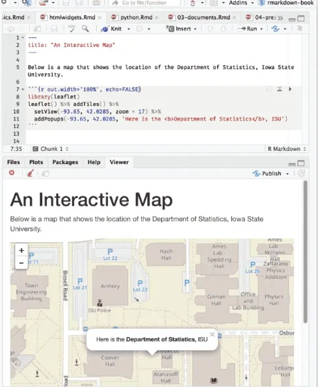
Figure 2.7 shows an interactive map created via the leaflet package, and the source document is below:
---title: "An Interactive Map"
---Below is a map that shows the location of the Department of Statistics, Iowa State University.
```{r out.width='100%', echo=FALSE} library(leaflet)
leaflet() %>% addTiles() %>%
setView(-93.65, 42.0285, zoom = 17) %>% addPopups(
-93.65, 42.0285,
'Here is the <b>Department of Statistics</b>, ISU' )
FIGURE 2.7: An R Markdown document with a leaflet map widget.
Although HTML widgets are based on JavaScript, the syntax to create them in R is often pure R syntax.
If you include an HTML widget in a non-HTML output format, such as a PDF, knitr will try to embed a screenshot of the widget if you have installed the R package webshot (Chang 2017) and the PhantomJS package (via webshot::install_phantomjs() ).
2.8.2 Shiny documents
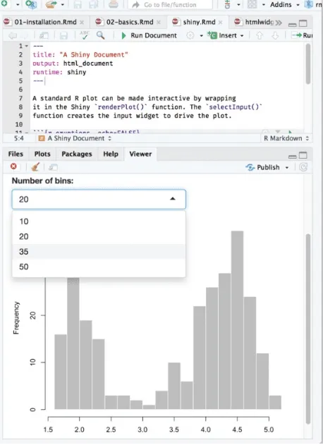
Figure 2.8 shows the output, where you can see a dropdown menu that allows you to choose the number of bins in the histogram.
---title: "A Shiny Document" output: html_document runtime: shiny
---A standard R plot can be made interactive by wrapping
it in the Shiny `renderPlot()` function. The `selectInput()` function creates the input widget to drive the plot.
```{r eruptions, echo=FALSE} selectInput(
'breaks', label = 'Number of bins:', choices = c(10, 20, 35, 50), selected = 20 )
renderPlot({
par(mar = c(4, 4, .1, .5)) hist(
faithful$eruptions, as.numeric(input$breaks), col = 'gray', border = 'white',
xlab = 'Duration (minutes)', main = '' )
FIGURE 2.8: An R Markdown document with a Shiny widget.
You may use Shiny to run any R code that you like in response to user actions. Since web browsers cannot execute R code, Shiny interactions occur on the server side and rely on a live R session. By comparison, HTML widgets do not require a live R session to support them, because the interactivity comes from the client side (via JavaScript in the web browser).
You can learn more about Shiny at https://shiny.rstudio.com.
HTML widgets and Shiny elements rely on HTML and JavaScript. They will work in any R Markdown format that is viewed in a web browser, such as HTML documents, dashboards, and HTML5
References
Vaidyanathan, Ramnath, Yihui Xie, JJ Allaire, Joe Cheng, and Kenton Russell. 2018. Htmlwidgets: HTML Widgets for R. https://github.com/ramnathv/htmlwidgets.
Xie, Yihui. 2018c. DT: A Wrapper of the Javascript Library ’Datatables’. https://rstudio.github.io/DT.
Cheng, Joe, Bhaskar Karambelkar, and Yihui Xie. 2018. Leaflet: Create Interactive Web Maps with the Javascript ’Leaflet’ Library. https://CRAN.R-project.org/package=leaflet.
Vanderkam, Dan, JJ Allaire, Jonathan Owen, Daniel Gromer, and Benoit Thieurmel. 2018. Dygraphs: Interface to ’Dygraphs’ Interactive Time Series Charting Library.
https://CRAN.R-project.org/package=dygraphs.
Chang, Winston. 2017. Webshot: Take Screenshots of Web Pages. https://CRAN.R-project.org/package=webshot.
Chapter 3 Documents
The very original version of Markdown was invented mainly to write HTML content more easily. For
example, you can write a bullet with - text instead of the verbose HTML code <ul><li>text</li>
</ul> , or a quote with > text instead of <blockquote>text</blockquote> .
The syntax of Markdown has been greatly extended by Pandoc. What is more, Pandoc makes it possible
to convert a Markdown document to a large variety of output formats. In this chapter, we will introduce the
features of various document output formats. In the next two chapters, we will document the presentation