Accelerated Source Sweep Analysis Using

1

Accelerated Source-Sweep Analysis using a

Reduced-Order Model Approach

Patrick Bradley, Conor Brennan, Marissa Condon, and Marie Mullen.

Abstract—This paper is concerned with the development of a model-order reduction (MOR) approach for the acceleration of a source-sweep analysis using the volume electric field integral equation (EFIE) formulation. In particular, we address the prohibitive computational burden associated with the repeated solution of the two-dimensional electromagnetic wave scattering problem for source-sweep analysis. The method described within is a variant of the Krylov subspace approach to MOR, that captures at an early stage of the iteration the essential features of the original system. As such these approaches are capable of creating very accurate low-order models. Numerical examples are provided that demonstrate the speed-up achieved by utilising these MOR approaches when compared against a method of moments (MoM) solution accelerated by use of the Fast Fourier Transform (FFT).

I. INTRODUCTION

T

HE solution of electromagnetic wave scattering prob-lems, from inhomogeneous bodies of arbitrary shape, is of fundamental importance in numerous fields such as geoscience exploration [1] and medical imaging [2]. For such problems, it is common to require the repeated solution of the electromagnetic wave scattering problem for a variety of source locations and types. This is of particular importance in the reconstruction of unknown material parameters in inverse problems and as such is a critical step in the optimisation process [3].

Typically, the relevant integral equation (IE) is discretised using the MoM and results in a series of dense linear equa-tions. The computational burden associated with the repeated solution of the full-wave scattering problem at each source location is severe, especially for large scatterers. Different strategies are used to accelerate the solutions of these linear systems. Considerable progress has been made in incorporat-ing sparsification or acceleration techniques [4] and precondi-tioners into iterative methods which permit expedited solutions of the scattering problem. The CG-FFT solution in particular is often applied in situations where the unknowns are arranged on a regular grid.

An alternative approach is to develop approximate solutions to expedite the solution of EM scattering problems. Several approximations of the integral equation formulation are dis-cussed in literature, including the Born approximations [5] and the family of Krylov subspace model order reduction techniques [6]. Although the Born approximation has been shown to efficiently simulate the EM response of dielectric

The authors are with the RF modelling and simulation group, The RINCE Institute, School of Electronic Engineering, Dublin City University, Ireland, (e-mail: bradleyp@eeng.dcu.ie and brennanc@eeng.dcu.ie)

bodies, these techniques are restricted to problems of relatively low frequencies and low contrast [5].

Krylov subspace approaches such as the Arnoldi algo-rithm [7]–[11] can produce very accurate low-order models since the essential features of the original system are captured at an early stage of the iteration. A set of vectors that span the Krylov subspace are used to construct the reduced order matrix model. By imposing an orthogonality relation among the vectors, linear independence can be maintained1 _{and so} high-order approximations can be constructed.

In this work, we modify the Arnoldi MOR procedure, in-troduced in [7], to efficiently perform scattering computations over a wide range of source locations for objects of vary-ing inhomogeneity. We consider a two-dimensional dielectric object characterised by permittivity ǫ(r_{) and permeability µ}

for a TMz _{configuration. A time dependence ofexp (ωt) is}

assumed and suppressed in what follows. The corresponding integral equation can be expressed in terms of the unknown scattered fieldEs

z(r)and total fieldEz(r)[13]

Ezs(r) =



4

Z

V

H₀(2)(kb|r−r

′

|)O(r′ )Ez(r

′ )dv′

(1)

whereO(r′

)is the object function at point r′

given by

O(r′

) =k2(r′

)−kb2. (2)

The background wave number is given by kb while k(r′)

is the wave number at a point in the scatterer.H₀(2) is the zero order Hankel function of the second kind. Usingmpulse basis functions and Dirac-Delta testing functions [13], Equation 1 is discretised by employing the MoM2_{, which results in the} following matrix equation

(I₊GA₎x₌b ₍₃₎

where b _{is the incident field vector at the centre of each}

basis domain, I _{is an m × m identity matrix and} G _is

an m×m matrix containing coupling information between the basis functions. A _{is an m×m diagonal matrix whose}

diagonal elements contain the contrast at the centre of each basis domain

ζmm=

ǫ(r′

m)

ǫb

−1. (4)

We note that for large scatterers Equation 3 cannot be solved by direct matrix inversion.

1_{Note that due to finite precision computation loss of orthogonality between}

the computed vectors can occur in practical applications [6], [8], [12].

2_{Note that other basis and testing functions are possible without affecting}

2

II. THE ARNOLDI ITERATION

The Arnoldi algorithm is an orthogonal projection method that iteratively builds an orthonormal basis for the Krylov subspace Kq [8]

Kq(G,u1) =span{u1,Gu1,· · ·,Gq

−1_u

1} (5)

for G_{generated by the vector}u_{1. This algorithm generates a}

Hessenberg reduction

H_{q =}UH

q GUq (6)

where H_{q is an upper Hessenberg matrix [8]. Note that the}

subscript q is used to denote a q×q matrix, where q≪m, the order of the MoM matrix. The columns of

U_{q = [}u_1,u_{2,· · ·,}u_{q] (7)}

are derived iteratively using the Arnoldi process in Table I [8].

u_{n are termed the Arnoldi vectors and they define an}

or-thonormal basis for the Krylov subspace Kq(G,u1). The

Arnoldi procedure can be essentially viewed as a modified Gram-Schmidt process for building an orthogonal basis for the Krylov space Kq(G,u1). The unit vectors un are mutually

orthogonal and have the property that the columns of the generatedU_{q matrix span the Krylov subspaceKq. Critically,}

the Arnoldi iteration can be stopped part-way, leaving a partial reduction to Hessenberg form that is exploited to provide a reduced order model (ROM) for Equation 3.

It should be noted that the choice of start vectoru_{1is critical}

in the early extraction of eigenvalue information of G_{. As}

such, one should attempt to construct a start vector that is dominant in the eigenvector directions of interest. In theory,

w_{n (line 9 Table I) will vanish if} u_{1 is a linear combination}

ofqeigenvectors ofG_{. In the absence of superior information}

we choose the initial incident field as the start vector u_1.

Indeed it has been shown experientially that a random vector is a reasonable choice [8], [14]. In the context of a source sweep analysis, our choice of start vector has no bearing on the accuracy of the approximation at other source locations. We do not discuss practical error controls in this paper but instead direct the reader to [6], [8], [14], where the topic is presented in detail. Suffice to say, that these techniques are applicable in what follows.

III. METHODOLOGY

In a source sweep analysis, the computation of the scattered fields from an inhomogeneous body requires independently solving

x_{= (}I₊GA₎−1_b

(8)

for each step in source location. The Arnoldi algorithm produces a ROM by iteratively computing the Hessenberg reduction

H_{q =}UH_q GU_q. (9)

Afterq steps of the Arnoldi algorithm, an approximation x_q,

tox_{, can be made in terms of the qbasis vectors}

x_≈x_{q =}

q

X

n=1

u_nαn=U_qa_{q (10)}

TABLE I

ARNOLDI-MODIFIEDGRAM-SCHMIDT ALGORITHM WITH

RE-ORTHOGONALISATION(MGSR).

Input: MatrixG, number of stepsq

and orthogonalisation parameterη= 1/√2,

u1=b/kbk2 for n= 1, . . . , q

w_n=Gu_n

vn=kw_nk2

for i= 1, . . . , n yi,n=uH

i wn

wn=wn−uiyi,n

endi

if kwnk2< η∗vn for i= 1, . . . , n hi,n=uT

iwn

w_n=w_n−uihi,n

endi

hn,n=hn,n+yn,n

endif

hn+1,n=kwnk2 ifhn+1,n= 0Quit

u_n+1=wn/hn+1,n

endn.

H=h(1 :q,:)

where a_{q = [α1 α2 · · · αq]}T _{is a vector of expansion}

coefficients for the Arnoldi basis vectors u_{n that span the}

Krylov subspace. The residual r_{q that corresponds to this}

approximation is introduced as

r_{q =}b₋₍I_m+GA₎x_{q. (11)}

To find the optimal approximate solution, x_{q is constrained}

to ensure thatx_{q minimises the residual}r_{q. Specifically, the}

residual vector is constrained to be orthogonal to theqlinearly independent vectors u_{q. This is known as the orthogonal}

residual property, or a Galerkin condition

r_{q ⊥ Kq or} UH_q r_{q = 0. (12)}

The residual r_{q is minimised when the residual vector is}

orthogonal to the space Kq. This requires substituting

Equa-tion 10 into EquaEqua-tion 11

r_q=b₋₍I₊GA₎U_qa_{q (13)}

and performing a Galerkin test, to give

UH_q r_{q =} UH_{q (}b₋₍I₊GA₎U_qa_{q) (14)} = UH_q b₋¡_I

q+UHq GAUq¢aq (15)

≈ UH_q b₋¡I_q+U_qHGU_qUH_q AU_q¢a_{q (16)} = UH_q b₋³I_q+H_qA˜_q×q

´

a_{q (17)}

where

˜

A_{q =} UH_q AU_{q. (18)}

As a result of setting

a_{q =}³I_q+H_qA˜_q´ −1

UH_q b ₍₁₉₎

the residual has been minimised as

UH_q r_{q =}UH_q b

−³I₊H_qA˜_q´ ³I_q+H_qA˜_q´ −1

3

yielding the following ROM for the total field

x_≈x_q=U_q³I_q+H_qA˜_q´ −1

UH_q b. (21) The key advantage is that once the Krylov matrix U_{q has}

been generated and stored the matrix I_{q +}H_qA˜_{q can be}

rapidly created and stored, along with its inverse permitting the solution for multiple right hand side vectors, even in the case of large scatterers as typically q≪m.

It should be noted that the step from Equation 15 to Equation 16 is, in general, approximate. It is exact only if the rangeR(U_q)ofU_{q is an invariant subspace of}A_{. However,}

due to the independence of the columns of U_{q imposed by}

the re-orthogonalisation process, this step can be shown to be a very reasonable approximation. As prescribed in [8], if the columns of U_{q are independent and the norm of the residual}

matrix

R₌AU_q−U_qS_{q (22)}

has been minimised for some choice ofS_{q, then the columns}

of U_{q define an approximate subspace. The selection of} S_{q =} UH_q AU_{q = ˜}A_{q results in the norm of the residual}

being minimised

minkAU_q−U_qS_qk2=k¡_I

−U_qUH_q ¢_AU

qk2. (23)

Thus, Equation 16 becomes a valid approximation with the property that, asq→m, a better approximation is procured.

IV. RESULTS

In this section, the monostatic radar cross section (RCS) is calculated from various geometries for a variety of source locations with a fixed contrast profile. The numerical perfor-mance of the reduced order model, generated using the Arnoldi algorithm, is compared against a MOM solution using an FFT-accelerated solver.

A. Case Study I

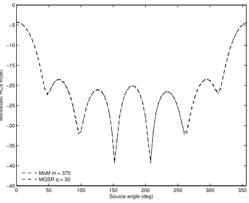
We initially consider a homogeneous cylinder embedded in free space. It is centred at the origin with radiusr= 0.6λand discretised using m= 370cells. The structure is illuminated by a transverse magnetic (TMz) wave emanating from a line source located at (10 cosφ,10 sinφ) where φ varies in the range 0 : 2πat increments of 8◦

. The assumed frequency is f = 300 MHz and the cylinder contrast is fixed at ζ = 1.5

(ǫr= 2.5).

Figure 1 depicts the monostatic RCS obtained from the MoM and the modified Gram-Schmidt algorithm with re-orthogonalisation (MGSR) technique presented in this paper, for q = 30, representing a 92% reduction in system size. The MGSR technique achieves an RCS average error (AE) of 0.12dB over the entire source range, while yielding a RCS maximum error (ME) of 0.72dB.

0 50 100 150 200 250 300 350

−45 −40 −35 −30 −25 −20 −15 −10 −5 0

Source angle (deg)

Monostatic RCS

σ

(dB)

MoM m = 370 MGSR q = 30

Fig. 1. Case Study I: Monostatic RCS from an homogeneous circle with constant contrast and varying source location.

B. Case Study II

We now consider an inhomogeneous layered scatterer with square cross section centred at the origin, with side length l= 3λembedded in free space. We assume the square to be composed of four equally sized slices each with widthwi =

0.75λand heighthi= 3λ. The number of basis functions used

is m = 3030 with fixed contrast values of ζ1 = 4, ζ2 = 3,

ζ3= 2 andζ4= 1.1. The monostatic RCS is again computed

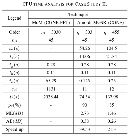
for the same range of line source locations as before. The MGSR technique achieves an impressive reduction in system size while yielding an acceptable AE over the entire source range. This is highlighted in Figure 2, which compares RCS obtained from the MoM and the MGSR technique for q = 455 representing a 85% reduction in system size. A complete CPU time analysis associated with the solution of the RCS for the FFT-accelerated MoM, and MGSR for ns= 45 samples is given in Table II. Within this table tu is

representative of the time3 taken to generate the Krylov U_q

matrix. Similarly, ti refers to the time taken to generate the

initial A˜_{q, tg refers to the time taken to generate the FFT}

component ofG_{, andtb refers to the time needed to generate} b_{.tsis the average time taken to solve the monostatic RCS at}

each source location using CGNE or CGNE-FFT accordingly. ni = number of iterations taken by the solver in order to

reach the tolerance10−5_.t

tis the total time taken to generate

and solve case study problem andpr = ROM size reduction

expressed in %. These simulations were run on a 3.00 GHz Xeon CPU processor with 3.00 GB of RAM at 2.99 GHz and the MoM solution is solved using the Conjugate Gradient Normal Equation method accelerated with the Fast Fourier Transform (CGNE-FFT). The CGNE-FFT can reduce the cost of matrix vector multiplications from O¡

m2¢ operations per iteration toO(mlog₂m)operations.

It is evident from Table II, that the MGSR algorithm can significantly decrease the computational expense associated

4

0 50 100 150 200 250 300 350

−45 −40 −35 −30 −25 −20 −15 −10 −5 0 5

Source angle (deg)

Monostatic RCS

σ

(dB)

MoM m = 3030 MGSR q = 455

Fig. 2. Case Study II: Monostatic RCS from an inhomogeneous square with constant contrast and varying source location.

with the direct solution for each source location in a source sweep analysis. The main computational cost of this approach is incurred in generating the Krylov matrixU_{q and the initial}

contrast profile matrix A˜_{q. Note that these computations can}

also be accelerated using the FFT and, once generated, the

U_{q and}A˜_{q matrices can be reused in subsequent simulations}

involving independent source locations. From Table II, it is clear that considerable savings in CPU time can be achieved in a source sweep analysis by utilising the MGSR method. For a 85% reduction in system size (q = 455) using the MGSR method, the associated AE and ME’s are 0.26 and 1.46dB respectively over the entire source range. While errors of ME = 2.73dB and AE = 0.38dB are observed for a 90%reduction. It is also shown in Table II, that for 45 source locations (ns= 45)

the ROM obtained using the MGSR technique is 21.3 times faster in producing a solution for the RCS, than the CGNE-FFT method applied to the MoM matrix system. Note that the CGNE method was used to compute the unknown field in Equation 21 rather than direct inversion, in order to generate a conservative comparison.

V. CONCLUSION

We have presented a new method for accelerating source sweep analysis based on an extension of the Arnoldi MOR approach. Notably, we have shown that the Arnoldi algorithm can produce accurate low-order approximations for a relatively low computational cost. Using case studies, we demonstrated that the Arnoldi technique can produce a significant reduc-tion in the system size while still resulting in an accurate approximation over a wide source range. In addition we have demonstrated the computational saving achieved by using MOR techniques in the solution of scattering problems, when compared to techniques which are based on solving the MoM system using FFT-accelerated iterative solvers.

TABLE II

CPUTIME ANALYSIS FORCASESTUDYII.

Legend Technique

MoM (CGNE-FFT) Arnoldi MGSR (CGNE)

Order m= 3030 q= 303 q= 455

ns 45 45 45

tu(s) - 54.26 104.5

ti(s) - 14.06 21.84

tg(s) 0.28 0.28 0.28

tb(s) 0.11 0.11 0.11

ts(s) 65.29 0.125 0.25

ni 1131 11 12

tt(s) 2938.44 74.34 137.98

pr(%) - 90 85

ME(dB) - 2.73 1.46

AE(dB) - 0.38 0.26

Speed-up - 39.53 21.3

REFERENCES

[1] T. J. Cui, W. C. Chew, and W. Hong, “New approximate formulations for em scattering by dielectric objects,”IEEE Transactions on Antennas and Propagation, vol. 52, no. 3, pp. 684–692, March 2004.

[2] Q. H. Liu, Z. Q. Zhang, T. Wang, J. Bryan, and L. a. W. Ybarra, G.A.and Nolte, “Active microwave imaging. i. 2-d forward and inverse scattering methods,” IEEE Transactions on Microwave Theory and Techniques, vol. 50, no. 1, pp. 123 – 133, January 2002.

[3] T. Hohage, “Fast numerical solution of the electromagnetic medium scattering problem and applications to the inverse problem,”J. Comput. Phys., vol. 214, pp. 224–238, May 2006.

[4] W. C. Chew, E. Michielssen, J. M. Song, and J. M. Jin,Fast and Efficient Algorithms in Computational Electromagnetics. Norwood, MA, USA: Artech House, Inc., 2001.

[5] G. Gao and C. Torres-Verdin, “High-order generalized extended born approximation for electromagnetic scattering,” IEEE Transactions on Antennas and Propagation, vol. 54, no. 4, pp. 1243 – 1256, 2006. [6] E. J. Grimme, “Krylov projection methods,” Ph.D. dissertation,

Coordinated-Science Laboratory, University of Illinois at Urbana-Champaign, USA, Urbana-Urbana-Champaign, IL, 1997.

[7] N. Budko and R. Remis, “Electromagnetic inversion using a reduced-order three-dimensional homogeneous model,” Inverse Problems, vol. 20, no. 6, pp. S17–S26, 2004.

[8] G. H. Golub and C. F. Van Loan, Matrix Computations, 3rd ed. Baltimore, MD, USA: Johns Hopkins University Press, 1996. [9] O. Farle and R. Dyczij-Edlinger, “Numerically stable moment matching

for linear systems parameterized by polynomials in multiple variables with applications to finite element models of microwave structures,”

Antennas and Propagation, IEEE Transactions on, vol. 58, no. 11, pp. 3675 –3684, 2010.

[10] M. Zaslavsky and V. Druskin, “Solution of time-convolutionary maxwell’s equations using parameter-dependent krylov subspace reduc-tion,”J. Comput. Phys., vol. 229, pp. 4831–4839, June 2010. [11] D. Weile, E. Michielssen, and K. Gallivan, “Reduced-order modeling of

multiscreen frequency-selective surfaces using krylov-based rational in-terpolation,”Antennas and Propagation, IEEE Transactions on, vol. 49, no. 5, pp. 801 –813, May 2001.

[12] K. Gallivan, E. Grimme, and P. Van Dooren, “A rational Lanczos algorithm for model reduction,”Numerical Algorithms, vol. 12, no. 1–2, pp. 33–63, 1996.