Hydraulic and Hydrologic Modeling of Steep Channel of Putih River,
Magelang District, Central Java Province, Indonesia
Adi Putri Anisa Widowati
Master of Engineering in Natural Disaster Management, Universitas Gadjah Mada, INDONESIA [email protected]
ABSTRACT
Hydrologic and hydraulic modeling are important to be conducted to examine the watershed response based on a rainfall input, especially over disaster-prone watershed such as Putih River watershed in Magelang, Central Java Province. A GIS-based grid-based distributed rainfall-runoff model was used to simulate the rainfall-runoff transformation. A two-dimensional hydrodynamic flow modeling was then carried out to simulate the flood processes on the stream and floodplain area. A sensitivity analysis was conducted on infiltration rate, Manning’s n value, and rainfall intensity. Infiltration rate, Manning’s n value, and rainfall intensity give considerable effects to the resulted flow hydrographs. The modeling results show that the results of hydrologic-hydraulic modeling is in good agreement with the observed results.
Keywords
: Hydrologic-hydraulic model, rainfall-runoff model, two-dimensional hydrodynamic model.1 INTRODUCTION
The development of Geographic Information System (GIS) has a significant impact on hydrologic and hydraulic modeling. As GIS-based hydrologic and hydraulic data are now widely available, many recent hydrologic and hydraulic models have been developed based on GIS. Lahar flood occur regularly in Putih River, Central Java Province. Since the upstream is located near the peak of active volcano Merapi, Putih River has a huge amount of lahar producing sediment materials on its upstream. Located on the steep upstream, the sediment materials, when saturated by rainfall, have a high probability to produce destructive lahar flood threatening the populated downstream area. This research is aimed to assess the lahar flood in Putih River by applying a whole modeling process ranging from hydrologic modeling to hydraulic modeling.
2 HYDROLOGY AND HYDRAULIC MODEL
Zhang and Savenije (2005) simulated saturation overland flow by relating the variable source area to both the topography and groundwater level. Koren, et al. (2005) evaluated the performance of a grid-based distributed hydrology model when transforming rainfall to stream flow which resulted in runoff volumes that was in good agreement with the observed data. Liu, et al. (2009) modeled runoff volume and peak discharge based on several flood events using grid-based distributed kinematic hydrological model with rainfall data derived from climate radar. The research was able to reproduce
peak discharge conforming to the field observed data, and also show that the model can be used to evaluate the effect of change in land cover and soil on the stream flow due to human activity.
Miyata, et al. (2014) examined the effects of intensive local rainfall on flashflood events using a grid based distributed hydrological model. The hydrology model is able to both evaluate the basin response due to rainfall, in form of flow, and to identify contributions of each sub-basins to the quickly rising stream discharge.
3 THEORETICAL BASE
3.1 Watershed
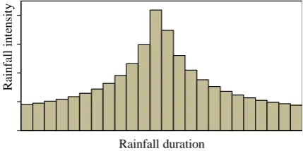
Table 1. Categorization of river bed-slope steepness develop hypothetical rainfall distribution, one of which is Alternating Block Method (Chow, et al., 1988). The general shape of design hyetograph by ABM is shown in Figure 1.
Figure 1. The design hyetograph derived by Alternating Block Method (ABM).
In Japan, the equation to calculate rainfall intensity for any duration based on daily rainfall depth is as follow (Mori, et al., 2003): storm (Chow, et al., 1988). The rising limb is the limb that has a positive gradient indicating the rising of discharge (point A to B). The recession limb is the limb that has a negative gradient indicating the falling of discharge (point B to C). Point C to D represents baseflow recession. Lag time between peak rainfall and peak discharge indicates the time required for a surface runoff flow to reach an outlet point where the hydrograph is observed. The shape of the hydrograph describes the response of a basin toward a rainfall
input which is different to another depending on several climatic, topographic, and geological factors.
Figure 2. The flow hydrograph at a basin outlet during a rainfall-runoff simulation by a particular observed rainfall event
3.4 Hydrologic – Hydraulic Model
Precipitation contributes to various storage and flow processes. The precipitation which becomes streamflow may reach the stream by overland flow, subsurface flow, or both (Chow, et al., 1988).
The passage of overland flow into a channel can be viewed as a lateral flow. A discharge of the overland flow, q0 per unit width, passes into the channel, with
the length of the channel, Lc, so the discharge in the
channel is Q = q0 Lc. To find the depth and velocity at
various points along the channel, an iterative solution of Manning’s equation is necessary.
2 roughness coefficient, R is hydraulic radius (m), and S is energy line gradient.
Infiltration is the process of water penetrating from the ground surface into the soil. Many factors influence the infiltration rate, including the condition of the soil surface and its vegetative cover, the properties of the soil, such as porosity and hydraulic conductivity, and the current moisture content of the soil (Chow, et al., 1988).
Hydrologic-hydraulic model is used to model rainfall-runoff transformation. The output of the model is flow hydrograph at a particular basin outlet. The model is a grid-based distributed model and consists of two domains. The first domain is hillslope and the second one is stream. The calculation in hillslope domain includes water balance calculation and flow routing on hillslope, while the calculation in stream domain consists of channel flow routing.
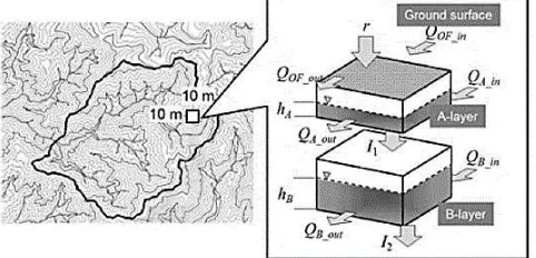
The scheme of hydrology model in hillslope domain is shown by Figure 2. In each grid, there are 3 layers on which runoff flow, sub-surface flow, and vertical flow between layers are calculated. The relation of a grid with its 8 surrounding grids is defined by flow direction. Flow direction of a grid to adjacent grid is determined by a grid whose elevation level is the lowest among those 8 surrounding grids.
Figure 3. The illustration of hydrologic model scheme on hillslope domain (Miyata, et al., 2014)
The illustration (Figure 3) explains the process of rainfall dropping on a surface of a hillslope grid which infiltrates to the layer A. The saturated flow of layer A then percolates to the layer B. The deeper percolation of flow on layer B to the deeper layer could occur, yet percolation flow to the deeper layer is assumed not flowing back to the slope or stream.
The hydrologic model calculates both runoff flow and lateral flow based on Manning equation and Darcy’s law. The runoff flow calculation takes into account the water balance from rainfall, flow from adjacent upstream grid, and flow to adjacent downstream grid, infiltration flow to the lower layer, and evaporation. The relation between depth of surface runoff flow, hOF, and runoff discharge per unit width, qOF, is
represented in the following equations:
r layer B. The equation to calculate lateral discharge per unit width, qA, and the flow depth, hA, in layer A, are:
layer A, qin_B is infiltration flow from layer A to layer
B, iA is hydraulic gradient of flow in layer A, and KA is
permeability coefficient of layer A. The calculation of lateral flow discharge and flow depth in layer B uses the equation same as of the layer A (Miyata, et al., 2014).
Furthermore, the calculation of discharge on stream domain, qCH, uses the same kinematic wave model
which is being used in flow model in hillslope domain. The composition of stream grid is carried out as a series of cross sections with lateral coming from adjacent right and left grids. The following equation is used to calculate the flow in stream domain:
L
3.5 Two-Dimensional Hydrodynamic Model SIMLAR v1.0
SIMLAR is developed by Yogyakarta Sabo Centre in cooperation with Universitas Gadjah Mada (Hardjosuwarno, et al., 2012). The hydrodynamic model is used to model flow along a particular stream or channel. The flow which is modeled using SIMLAR is of debris flow type. The debris flow is calculated as a fluid unity of debris flow and suspended sediments. Some equations used in the model are described as follows.
To calculate the permanent flow velocity at a uniform channel cross section, Manning equation is used. Based on flow velocity from the Manning equation, flow discharge at a particular channel cross section is calculated using the following equation.
uA
Q
(9)where Q is flow discharge (m3/s), and A is flow area
For a non-permanent and non-uniform flow, the debris equations are developed considering the mass conservation principles and force and momentum conservation principles.
Mass conservation equation for two-dimensional flow is:
Force and momentum equation for two-dimensional flow is:
where H is depth of flow (m), M is flow discharge per unit width at x direction (m2/s), N is flow discharge per unit width at y direction (m2/s), g is gravity acceleration (m2/s), and τ is shear stress.
4 METHODOLOGY
4.1 Location of Study
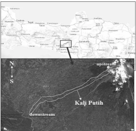
The research was carried out on Putih River watershed in Magelang District, Central Java Province. It has upstream end on the peak of Merapi Volcano. It flows downward the Merapi slope to the southwest direction until it intercepts with Blongkeng River on the downstream end. The boundary of Putih River watershed is shown by Figure 4.
Figure 4. Location of study area in Putih River watershed 4.2 Data Availability
a)
Topography data
Topography data for Putih River is LiDAR DEM of 20 m resolution which is obtained from Yogyakarta Sabo Center
b) Rainfall and water level data
Hourly rainfall data for Putih River watershed is obtained from Yogyakarta Sabo Center.
c) Physical simulation parameters
Several physical parameters for hydrologic-hydraulic simulation such as Manning coefficient and properties of bed material are collected from previous researches, namely Widowati (2015), and Musthofa (2014).
4.3 Research Tools
5 RESULTS AND DISCUSSIONS
5.1 Delineation of Putih River watershed
The result of the watershed delineation gives the total area of Putih River watershed (Figure 5) as 23.011 km2 with a total length of the main river of 21.639 km. The sub-watershed has an area of 8.432 km2. The sub watershed of Putih River has riverbed slope ranging from 3.0° to 7.6°.
Figure 5. The delineation of Putih River watershed and sub-watershed.
5.2 Rainfall – Runoff Modeling
The rainfall-runoff modeling is conducted using kinematic distributed model. The final results are flow hydrograph on the outflow point. A sensitivity analysis was conducted on infiltration rate, Manning’s n value, and rainfall intensity. The rainfall event used during the simulation of sensitivity analysis is the rainfall event on December 8th 2010 recorded at Ngepos station (Figure 6).
The simulated watershed boundary in Putih River covers Putih River upstream sub-basin with an outlet point located at approximately upstream of PUD-02.
The area of Putih River inflow sub-basin is 8.43 km2. Figure 7 presents the scheme of slope and stream domain of the simulation.
Figure 6. Rainfall event of December 8th 2010 in sensitivity analysis in Putih River.
Figure 7. The scheme of stream and watershed used in rainfall-runoff modeling in Putih River.
5.2.1 Sensitivity analysis on infiltration rate
The sensistivity analysis used a constant slope
Manning’s n = 0.7 and a constant channel Manning’s
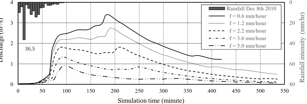
n = 0.03. Figure 8 shows the results of sensitivity analysis on infiltration rate in Putih River upstream watershed. Table 2 provides the values of the resulted peak discharge and peak time.
Figure 8. Simulated channel flow discharge hydrographs at outlet point using different values of infiltration rate in Putih River.
36,5
0
20
40
60
80
0 1 2 3 4
0 50 100 150 200 250 300 350 400 450 500 550
R
a
in
fa
ll
i
n
te
n
si
ty
(m
m
/h
r)
D
is
c
h
a
rg
e
(
m
3/s
)
Simulation time (minute)
Rainfall Dec 8th 2010 f = 0.6 mm/hour f = 1.2 mm/hour f = 2.2 mm/hour f = 3.6 mm/hour f = 5.0 mm/hour
Table 2. Peak discharge (Q) and and peak time (tp) of simulated hydrographs in sensitivity analysis of infiltration rate (f) in Putih River. runoff discharges. High infiltration rate also diminishes the discharge of flows from far-grids that enter the stream at a later time which is indicated by later peaks in the hydrographs of small infiltration rate. The later rising parts of the hydrographs of small infiltration rate (f = 0.6, 1.2, and 2.2 mm/hour) appear due to the flow from slope-grids located in farther distance from the stream that just enter the stream at a later time. In the hydrograph with high infiltration rate (f = 5.0 mm/hour), this additional rising part of hydrograph is not observed because the flow is already being infiltrated into the soil along its path to the stream. Small infiltration rate also gives flow a chance to accumulate faster, thus hydrograph of small infiltration rate rises earlier.
5.2.2 Sensitivity analysis on Manning’s slope n values
Referring to the Manning’s n value from literature study (Engman, 1986), the surface condition in Putih River is considered ranging from grass to woods.
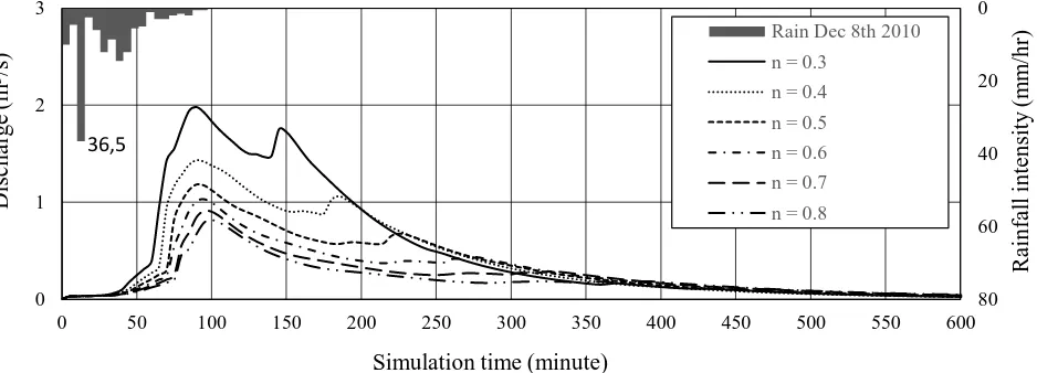
Thus, it was taken the Manning’s n values ranging from 0.3 to 0.8 for sensitivity analysis of Manning’s n value. The result of sensitivity analysis of Manning’s n values is shown by Figure 9. Table 3 provides the values of the resulted peak discharge and peak time.
Table 3. Peak discharge (Q) and peak time (tp) of simulated hydrographs in sensitivity analysis of infiltration rate (f) in Putih River. coefficient, smaller Manning’s slope n values results in higher flow velocity than higher n values. High flow velocity also gives effect in reducing the chance of the flow to be infiltrated into the soil. Thus, smaller n values produce greater and faster flow discharge entering the stream than higher n values.
In addition, small n value which results in high flow velocity is correlated with a faster draining time. Flow with high velocity is easier to be drained out of slopes than slow flow, thus makes it quicker for the flow both to form the peak discharge and to decline. So, small n value makes the hydrographs sharper: shorter duration to reach the peak discharge, higher peak discharge rate, and steeper recession limb.
Figure 9. Simulated channel flow discharge hydrographs at outlet point by different Manning’s slope n values in Putih River.
Figure 10. Comparison of the simulated channel flow hydrographs at outlet point by different hypothetical rainfalls in Putih River.
5.2.3 Modeling with variation of rainfall intensity
The design hyetograph was derived using a modified Mononobe equation and distributed using Alternating Block Method (ABM) technique. The results of modeling with variation of rainfall intensity in Putih River is shown in Figure 10. Although the infiltration
rate and Manning’s slope n value are set constant of f
= 5 mm/hour and n = 0.7 respectively, each rainfall produces different shape of hydrograph.
The hypothetical rainfall of P2-hours = 10 mm produces
a very low hydrograph with maximum peak discharge of 0.7 m3/s at t = 215 minute. The hypothetical rainfall P2-hours = 15 mm produces a terraced hydrograph with
a discharge rising at t = 180 min and a peak discharge rate of 3,541 m3/s at t = 285 minute. The hypothetical rainfall P2-hours = 20 mm starts to rise at t = 155
minutes and reaches maximum discharge rate 9,277 m3/s at t = 245 minutes. The hypothetical rainfall P 2-hours = 25 mm starts to rise at t = 145 minutes and
reaches maximum discharge rate 15.99 m3/s at t = 225 minute.
The hydrographs have different shape one another. The hydrographs of higher rainfall depth rise earlier have higher discharge. The maximum discharge also occurs earlier in the hydrographs of higher rainfall. By the specified rainfall distribution, the maximum discharge occurs after the rain stops. The rainfall intensity affects the flow discharge greatly, and produces hydrographs of rainfall intensity distinctly.
5.3 Hydrodynamic Modeling
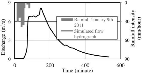
The hydrodynamic debris flow modeling was carried out on Putih River basin. The inflow point is assigned at the downstream of PUD-02. The downstream
boundary of the modeling is the upstream of PU-C0 Sukowati. The inflow hydrograph (Figure 11) was obtained from rainfall-runoff modeling in Putih River upstream sub-basin of January 9th 2011 rainfall event from Ngepos ARR station, using infiltration rate of f =
5 mm/hour and Manning’s slope n value of n = 0.7.
The hydrodynamic modeling of debris flow in Putih River was conducted for 210 minutes.
Figure 11. Inflow hydrograph for Putih River hydrodynamic modeling.
The result of hydrodynamic lahar modeling is a spread of water and sediment inundation on the simulated Magelang public road, at t = 180 minutes.
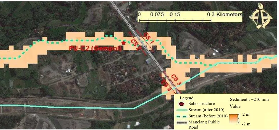
Figure 12. Simulated sediment spread of debris flow in Putih River at t = 210 minutes
Figure 13. Sediment inundation near Magelang public road.
Based on the simulation results of debris flow modeling until t = 210 minutes, the overtopping of water and sediment to the river side is not visually observed. Meanwhile, the velocity of water flow and sediment flow from simulation result is still too low compared to the field event. From the recorded event, when a lahar was triggered by a rainfall in the upstream of Putih River, the lahar flow reached the downstream near Magelang road within 1 hour (60 minutes). However, the simulation results show that the travel of water and sediment took 2 hour (120 minutes) to arrive at the downstream area near Magelang road.
One of the public facility vulnerable toward Putih River debris flow is Magelang public road located upstream of PU-C2 (Gempol). An image of sediment inundation near Magelang road is shown by Figure 13, in which two courses of Putih River reach are described, one is the old stream course before debris flow of Merapi 2010 eruption which is represented by a dashed line, and another one is the new stream course after the debris flow of Merapi 2010 eruption represented by a continuous line.
According to the field report of debris flow occurrence prior to Merapi eruption in
October-Sabo structure Stream (after 2010) Stream (before 2010) Magelang Public Road
Sediment t =210 min Value
2 m
November 2010, the debris flow in Putih River overtopped to and inundated the Magelang road several times, one of which was the debris flow occurrence at January 9th 2011. The new stream course was formed due to the huge and massive force of the debris flow which overtopped the road. However, the simulated results indicated that debris flow based on rainfall of January 9th 2011 remained through the old stream course. Some part of the flow seemed to start entering the new stream course. It may be caused by the lack of DEM resolution which was 20 m. A hydrodynamic modeling of lahar flow using DEM with smaller resolution which more represents river topography should be conducted to have a more accurate result.
Four cross-sectional stream profiles (CS 1, CS 2, CS 3, and CS 4) at the Putih River reach which intersects Magelang public road are extracted to observe the effect of sediment erosion and inundation near the vulnerable public road. Figure 14 shows the riverbed changes due to sediment erosion and sediment inundation at the specified cross-sectional stream profiles. The cross-sectional stream profiles are extracted at t = 180 minutes and t = 210 minutes only based on the time the sediment flow has reached the Magelang road.
At CS 1, it is observed that an erosion occurs with the maximum erosion depth of 0.73 m at t = 210 minutes. The riverbed has been lowered due to the erosion. At CS 2, it is observed that a sediment inundation occurs with the maximum sediment inundation depth of 0.20 m at t = 210 minutes. At CS 3, it is observed that a sediment inundation occurs with the maximum sediment inundation depth of 0.49 m at t = 210 minutes. At CS 4, it is observed that a sediment inundation occurs with the maximum sediment inundation depth of 0.94 m at t = 210 minutes.
6 CONCLUSIONS AND RECOMMENDATIONS
6.1 Conclusions
Several conclusions of this research are:
a) Infiltration rate affects the magnitude of flow discharge. The higher infiltration rate, the lower the resulted runoff flow discharge. Infiltration rate also affects the shape and peaks hydrograph
b) Manning’s n value affects the flow velocity. The
small Manning’s n value results in fast
-accumulated flow and high discharge.
c) Rainfall intensity dominantly affects the typical hydrograph, yet, the effect of rainfall intensity toward the hydrograph parameter is different from one rainfall intensity and other intensities.
6.2 Recommendations
Of all the research results, there are several recommendation for a better future research:
a) The rainfall-runoff model should be applied on basins with different topography and stream structure, such as basins with finer slope and more stream tributaries.
b) The radar-derived rainfall data should be applied as rainfall input in order to produce a spatially better result.
c) A hydrodynamic modeling of lahar flow using DEM with smaller resolution should be conducted to have a more accurate result.
d) A longer duration of hydrodynamic modeling of lahar flow should be conducted to observe the longer debris flow propagation over a stream reach.
REFERENCES
Chow, V. T., Maidment, D. R. & Mays, L. W., 1988. Applied Hydrology. New York: McGraw-Hill, Inc.. Delson, 2012. Kajian Lahar Hujan Kali Putih Setelah Letusan Gunungapi Merapi 2010 [Study on Lahar at Putih River after Merapi Eruption 2010], Yogyakarta: Faculty of Engineering, Universitaws Gadjah Mada.
Engman, E. T., 1986. Roughness coefficients for routing surface runoff. Journal of Irrigation Drainage Engineering, 112(1), pp. 39-53.
Hardjosuwarno, S. et al., 2012. Panduan Pengoperasian Program Simulasi 2D Banjir Debris SIMLAR Veris 1.0.2011 [Guideline fo 2Dr Debris
Flow Simulation SIMLAR Version 1.0.211], Yogyakarta: Sabo Office.
Hardjosuwarno, S. et al., 2012. Panduan Pengoperasian Progra m Simulasi 2D Banjir Debris Veris 1.0.2011. Yogyakarta: Balai Sabo Yogyakarta. Koren, V. et al., 2005. Evaluation of a grid-based distributed model over a large area . BrazIAHS Scientific Assembly.
Liu, J., Feng, J. & Otache, M. Y., 2009. A grid-based kinematic distributed hydrological model for digital river basin. In Advances in Water Resources and Hydraulic Engineering. Heidelberg ed. Berlin: Springer.
Miyata, S., 2014. Manuals of Simulation Program for GIS Based Rainfall-Runoff Model, Kyoto: Kyoto University.
Miyata, S., 2014. Manuals of Simulation Program for GIS Based Rainfall-Runoff Model, Kyoto: DPRI Kyoto University.
Mori, K., Ishii, H., Somatani, A. & Hatakeyama, A., 2003. Hidrologi untuk Pengairan [Manual on Hydrology]. 9th ed. Jakarta: Paradnya Paramita. Musthofa, A., 2014. Simulasi Banjir Bandang untuk Peringatan Dini dan Bahaya, Yogyakarta: Gadjah Mada University.
Rosgen, D. L., 1994. A classification of natural rivers. Catena, 22(2), pp. 169 - 199.
Shusuke, M., Masaharu, F., Takuji, T. & Tsujimoto, H., 2014. Flash Flood due to Local and Intensive Rainfall in an Alpine Catchment. Nara, International Sabo Association.
SID Jumoyo, 2015. Sistem Informasi Desa (SID) Jumoyo, Kecamatan Salam, Kabupaten Magelang. [Online]
Available at: http://jumoyo-magelang.sid.web.id [Accessed June 2017].