Automatic Global Optimal Estimation of Large Residual Statics
Rey-Villamizar, N.∗, and Yilmaz, O., Paradigm Geophysical
SUMMARY
In this paper we present an algorithm to estimate a global max-imum for a large scale residual statics problem in an automatic manner. We model the problem as a maximization of a cost function. Our specific formulation of the problem allows us to efficiently find upper and lower estimates of the optimal solu-tion. This property of our formulation also enables the use of a Branch and Bound (B&B) algorithm design paradigm to solve the combinatorial optimization problem of large scale residual statics. Our formulation is also efficient in that each branch instance produces different candidate solutions. In contrast to previously proposed solutions of the global optimization prob-lem, such as simulated annealing, our solution to the residual statics estimation problem is guaranteed to be within an in-terval of the estimated global optimal solution. We use our proposed formulation of the problem to find the solution of the stack problem that maximizes the stack power or that mini-mizes the variance.
INTRODUCTION
Land seismic data is distorted by the near-surface inhomo-geneities that are too small to be modeled or accounted for in wave propagation. Their impact is mitigated by estimating a time invariant correction for each source and receiver in a surface-consistent manner (Ronen and Claerbout (1985)). Ad-ditional axes can be added to the problem, such as common midpoint, common offset, residual moveout etc. (Taner et al. (1991)). Most of todays publications and implementations ei-ther seek a localized solution of the global problem or a simple linearized solution of this highly non-linear task. Linearized versions mainly rely on iterative enhancement of a pilot trace, either taken as an input or estimated in an iterative manner. Conventional methods fail to compute very large statics due to, among other things, the difficulty to construct a good pilot trace. A good pilot trace is a trace that in the iterative methods can lead to the global solution.
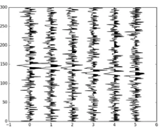
As an example, take the global solution of the maximum stack power problem. Considering all the combinations, it is an enormous and impossible task to solve. Simply consider a sin-gle CDP gather of 6 traces with a maximum shift of 21 sam-ples, as in Figure 1. To examine all the possible combinations, the number of shift settings that need to be tested is(21)6. The number of combination to evaluate increments exponentially with respect to the number of traces. Furthermore, consider that these combinations must be extended to a region of CDPs that are covered by the extent of common shot and common receiver gathers, for a surface-consistent solution. The task is simply too hard to solve with today’s computers in a reason-able amount of time, even for a single CDP and small number of static shifts. Rothman (1986) attempted to devise a global solution using a modified version of the Monte Carlo approach.
Figure 1: Syntetic traces with static shift. Testing all the pos-sible combinations for maximum shift of 21 samples requires to evaluate 8.5 billion possibilities.
They used a “heat bath” method in which the next point is chosen in the parameter space with the maximum Gibbs prob-ability. They used stack power as the objective function. Va-sudevan et al. (1991) used simulated annealing, which showed improved results over linearized methods. Simulated anneal-ing has three main parts, one of which is temperature—itself a difficult parameter to estimate. In their work, Vasudevan et al., pointed out some of the limitations of formulating the prob-lem as a maximization of the stack power and used the coher-ence between the neighboring CDPs instead. The main draw-backs with all of the above-mentioned solutions are that, in most cases, they require parameters that are difficult to set up or they are not guaranteed to approximate the global solution but rather an approximation of a local solution.
In this paper we devise a formulation of the problem that al-lows efficient computation of lower and upper bounds of the global energy function. This functionality allows us to use the Branch and Bound (B&B) algorithm paradigm proposed by Land and Doig (1960) to optimize the energy function. This algorithm paradigm is a common tool for solving NP-hard op-timization problems. The B&B algorithm is an improvement over a brute-force enumeration of all the possible solutions in that it keeps track of the bounds of the objective that it is try-ing to find. It uses those bounds to “prune” the search space of regions that cannot contain solutions better than the current one. Our proposed approach can be used to solve many of the optimization problem using the B&B algorithm paradigm, including stack power, coherence between neighboring CDPs, etc.
THEORY AND METHODOLOGY
Automatic Global Optimal Estimation of Large Residual Statics
(Ronen and Claerbout (1985)):
Ti jk=Si+Rj+Gk+QkXi j2, (1)
whereSiandRjare the statics of theith source position and the
jth receiver position respectively,Gkis the structure term at the
kth CDP position,Qkis the residual NMO component at the
kth CDP, andXi jis the source-to-receiver distance normalized by the maximum distance in the survey.
These four terms constitute the unknowns of the statics inver-sion problem. The time shiftsTi j are usually found by using cross-correlation. A common solution to the problem is to cre-ate a pilot trace by stacking in CDP gathers, or super gathers (Ren et al. (2016)). However, in the presence of large statics in the input data, such an initial pilot trace may be insufficient to provide any useful cross-correlations which will lead the the global optimal.
Problem Formulation
We formulate the problem as Rothman (1985) did. Let the data recorded at the jth receiver, after theith shot has been fired at timet=0, be denoted byti j(t). Letfi j(t)be the same data but without noiseni j(t)and without static shift. Then,
di j(t) =Gi j(si,rj)fi j(t) +ni j(t) (2) where
Gi j(si,rj)fi j(t) =fi j(t−si−rj). (3) The problem is to estimate thesiandrjdirectly from the data. We formulate the problem of estimating the best shot and re-ceiver static shifts that willmaximizethe stack power in all CDP stacks. More formally: of CDP stacks. This is the function that we want to maximize.
Our methodology can also be used to maximize the coher-ence between CDPs, as proposed by Vasudevan et al. (1991). We will explain the required modification to our methodology to achieve this objective function. To formulate the problem, seismic traces are sorted to a midpoint-offset (y-h) coordinate and normal moveout corrected to produce the new set of traces
dyh(t). The inverse shifting operator in midpoint-offset coor-dinates is:
G−yh1dyh(t) =dyh(t+si(y,h)+rj(y,h)) =dyh(t+sri j(y,h)) (5) whereiand jare both functions ofyandh. We combine the termssi(y,h)+rj(y,h)intosri j(y,h)to simplify the notation in the losing generality, we set the range of static corrections for any shot-receiver, at mostPdifferent time-point shifts.
Methodology
Consider the case of one CDP, as in Equation (6). In this case, the energy of the stacked trace can be expressed as:
Ecd p(y) =
By changing the order of the summation, we get:
Ecd p(y) =
For a given offseth, the first term corresponds to the zero lag autocorrelation in the selectedTgate as a function of the time shiftsri j(y,h). In other words, the first term corresponds to the autocorrelation value with no lag. Subsequently, all the possible values of the first term for a given CDPy, can be stored in|O f(y)|vectors of sizeP, with P being the max-imum possible shifts of any given trace. In the same way, all the possible values of the second term can be reduced to |O f(y)|(|O f(y)|+1)/2≈ |O f(y)|2matrices of sizeP2. We can further reduce the number of values further by combining the two using an appropriate factor and adding the autocorre-lation row-wise (and column-wise).
In this formulation, any possible contribution of each pair of tracesdyhanddyh′ to the global energy function can be stored
by a matrix ofP2values. The problem of exploring the feasible space of solutions for a given time shift is reduced to regions of matrices that represent cross-correlations (multiplication and sum of two traces) for that shift. Computing lower and upper estimations of the cost function can be done by finding the minimum and maximum value of the appropriate regions of the matrix fulfilling a given constraint of a range of shifts.
The key observations in this formulation are:
• The global energy is a function of the summation of the
power of each trace and the pairwise correlation for all possible residual static ranges.
us to estimate lower and upper bounds in the energy for a given receiver or shot static.
• All the possible energy values for a given CDP can be
stored in|O f(y)|(|O f(y)|+1)/2≈ |O f(y)|2 number of matrices of sizeP2, wherePis the set of possible allowable time shifts.
• Computinglowerandupperbounds of the energy
func-tion for a given partifunc-tion of the space, consists of tak-ing the minimum or maximum respectively, of the set of regions of the matrices that include that particular range of values.
Computational cost of the initial set-up
One way of implementing the above-presented algorithm is by first computing the matrices of all possible time shifts between traces. After this step we only need to keep in memory these matrices to perform the optimization algorithm.
• Operations per CDP:|O f(y)|2P2|Tgate|
• Memory per CDP:|O f(y)|2P2
Branch and bound algorithm design paradigm
With the above presented formulation in Equation (8) we can use the Branch and Bound (B&B) design paradigm to solve the combinatorial problem of selecting the right statics correc-tion (Land and Doig (1960)). This algorithm paradigm is one of the main tools for solving hard combinatorial optimization problems. The B&B algorithm searches the complete space of solutions for the optimal solution. This approach is not a heuristic or approximate procedure, but it is an exact, op-timizing procedure that finds an optimal solution under cer-tain constraints. This algorithm is especially useful when it is impossible to enumerate the number of possible solutions due to the exponential growth of the number. This algorithm is comprised of three main components: selection of how to partition the solution space, efficient bounds calculation, and branching. The sequence of steps varies according to the strat-egy used to search the solution space. In our solution we use the so-calledeagersolution where-in bounds are computed as soon as a new node is available. Our formulation allows us to efficiently compute lower and upper bounds.
The bounding function is the most critical part of the B&B for-mulation. Astrongbounding function is one that more closely approximates the optimal solution; aweakbounding function has the opposite property. Unfortunately, in most cases there is always a trade-off between use of astrong(orweak) bound-ing function and computational time. We explain how we can compute bounds of different degrees ofstrengthin our formu-lation by trading computation efficiency.
Branching:Branching will be selected according to the pos-sible shifts of a given trace. A simple implementation will be: for each node, partition the set of possible trace shifts into two and compute the bound for each case. The partition can be made more granular depending on how the algorithm is imple-mented and which information is kept in memory versus on disk.
Bounding function: For a given traceT and a given range of shifts−∆p≤t≤∆q, the bounding values can be efficiently computed as the maximum (or minimum) of all the sub-matrices with that trace in one of its axis, which allows a shift on that range constraint by the current search space. This is a very “weak” bound. The bound value can also be explored on a column-by-column (or row-by-row) basis for the range of shifts. This is astrongerbounding function, however is also more ex-pensive operation.
This approach has very interesting theoretical and practical ad-vantages compared to the previously proposed solutions:
• Each iteration of the B&B algorithm approximates closer
to the global optimal solution.
• At any point in time, we guarantee to finding a solution
that is between estimated lower and upper bounds of the optimal solution.
• Given enough time, the algorithm can get as close as
possible to the estimated optimal solution.
• In general, the algorithm is not inherently parallel.
How-ever, some parts can be done in parallel. For example, the bounding function can be made verystrongand this part can run in parallel.
The use of the B&B paradigm for our proposed solution will work by keeping a priority queue (P) that uses the estimate of the best possible solution and the best current solution. We will use a variation of the algorithm called best-first B&B (Clausen (1999)), since we can obtain a good initial solution by using any of the linear methods to solve the problem, or just by us-ing an initial zero shift for all the traces. This approach will explore the space in a best-first search manner, exploring the feasible space with the best possible solution. The high-level description of a generic B&B algorithm works like this:
1. Find a good solution estimate and call it solution B.
2. For each trace, split the possible range of statics shifts into two, and compute the upper and lower bounds of each partition of the solution space. If the estimated cost of the upper bound is lower than the current so-lution B, then prune this part of the tree because we have already found a better solution than any possible solution in that part of the tree. Otherwise, add it to the priority queue.
3. Using the priority queue, select the partition of the space, with the best possible solution.
4. Repeat steps 2) and 3) until convergence criteria is ful-filled.
A convergence criteria could be finding a solution that is within a specific percentage of the best estimated bound. Another criteria could be a percentage over the best possible solution obtained in the first node of the solution tree.
Maximizing the coherence between CDPs
Automatic Global Optimal Estimation of Large Residual Statics
the maximum stack power to the coherence between CDPs. They justify their problem formulation by listing some of the limitations of maximizing the stack power, one of them being the fact that the relation between neighbor CDPs are not con-sidered. Our approach can be modified to solve this objective function, too. In this case, the objective function will still be the summation over all the CDPs. For a given CDP, the power will take the form:
Following the same derivations of Equation (8), we can now expand this objective function and we will need the cross-correlation between all the traces of one CDP with all the traces from the neighboring CDP. In other words, when we compute the stack power we are computing the power of two, and some of the correlations are repeated. In the objective function pro-posed by Vasudevan et al. (1991) there are no repeat of pair-wise cross-correlations, therefore the amount of computation is increased.
Constraining the solution
Our formulation of the problem also allows for the inclusion of constraints of the neighbor static shifts, which are straightfor-ward enough to include in the framework. For example, we can impose a smoothness constraint by exploring the state space of possible residual statics in such a way that for neighbor re-ceivers, the total residual static does not change more than a given value. Consider that, at any point in time, the partition of the search space can be described by−∆tq≤si+rj≤∆tp for everyiand j. We could impose constraints in the rela-tion of the residual statics with the neighbor shotsi+1and re-ceiverrj+1 by limiting the search space ofsi+1+rr+1to be within some constant of the current search space forsi+rj. The same can be applied for all the first-order, or even second-order, neighbors. These could be implemented in the branch-ing function of theB&Balgorithm.
Variance minimization
The above-presented algorithm can be used to also minimize the variance of the stack trace with respect to the pre-stack traces. We can modify Equation (8) by using the following formulation. Consider:
This represents the CDPyat timet divided by the number of different offsets for that CDP. From this, the variance with respect to the CDPycan be expressed as:
Var(CDPy) = X
where the term in the inner-most part of the summation has the same form as the Equation (8), but different only by one factor for each offset
The same derivation as in Equation (8) can be used to express this in matrix form, and the B&B algorithm can be used to explore the feasible set of solutions.
Conclusion
We have presented a formulation of the residual statics prob-lem that can give the global solution using the B&B algorithm paradigm. This is possible due to the fact that we can compute lower and upper bounds efficiently. Our method is also able to compute a bounding function that can be madestrongeror
weakerby using more computer cycles. We show how our for-mulation can be used to find the global optimum of the maxi-mum stack power problem within some estimated distance of the global optimum. We also show that our method can be used to find estimate and approximate the global optimum of two other cost functions. It can also be used find the minimum variance of the resultant trace with respect to the pre-stack data. Additionally, we show how it can also be used to approx-imate the solution of the maximum coherences between CDPs, as proposed by Vasudevan et al. (1991). Finally, we presented how our formulation can be modified to include smoothness constrains on adjacent shot-receiver neighbors. This is some-thing that we plan to investigate in more detail in our future work.
ACKNOWLEDGMENTS
Note: This reference list is a copyedited version of the reference list submitted by the author. Reference lists for the 2017 SEG Technical Program Expanded Abstracts have been copyedited so that references provided with the online metadata for each paper will achieve a high degree of linking to cited sources that appear on the Web.
REFERENCES