this PDF file Applying Fuzzy Analytic Hierarchy Process (FAHP) Cut Based and TOPSIS Methods to Determine Bali Provincial Road Handling Priority | D.M.P. | Civil Engineering Dimension 1 PB

(1)

Applying Fuzzy Analytic Hierarchy Process (FAHP)



-Cut Based

and TOPSIS Methods to Determine Bali Provincial Road Handling

Priority

Wedagama, D.M.P.1_{and Frederika, A.}1

Abstract: The Analytic Hierarchy Process (AHP) method has been employed in a previous study

to determine Bali provincial road handling priority. This method usually overlooks the decision

maker’s degrees of confidence and optimism of the decision. Meanwhile, Fuzzy Analytic Hierarchy Process (FAHP) -cut based and Technique for Order Preference by Similarity to Ideal Solution (TOPSIS) methods allow the researcher to estimate the overall road handling priority considering on degrees of confidence and optimism of the decision. The present study aims at determining Bali provincial road handling priority using FAHP -cut based and TOPSIS

methods. The current study shows that decision makers’ degree of confidence in both pessimistic

and moderate situations and optimism from certain to the most uncertain conditions suggesting the same road link as the highest priority compared to the previous study. Both current and previous studies also conclude the same road link as the lowest road handling priority.

Keywords: Road handling, fuzzy AHP -cut based method, TOPSIS.

_

Introduction

Road handling priority is deemed as a complicated multi-criteria decision making process. In so doing, various aspects including economics, relations among regions, accessibility, political considerations, defence, and security should be considered. In a previous study [1], the macro transportation system [2] was used to construct the main and sub criteria of the problem and the Analytic Hierarchy Process (AHP) was used to determine provincial road handling in Bali. The study suggested that the AHP is effective and logical in determining Bali provincial road handling priority.

The AHP method, however, may not entirely show a way of human thinking because the experts/decision makers typically tend to express interval judgments rather than sorts of single numeric values [3]. In addition, the AHP can not be entirely put into practice as it is usually overlooking the decision

maker’s degree of confidence and degree of optimism

of the decision. The pairwise comparison (PC) ratios in the AHP are in crisp real numbers [4] and decisions always consisting vagueness and variety of meaning. The descriptions of decision makers are typically linguistic and vague.

1 _{Department of Civil Engineering, Faculty of Engineering Udayana} University, Bukit Jimbaran–Bali, INDONESIA.

Email: priyantha_wedagama@googlemail.com

Note: Discussion is expected before November, 1st _{2011, and will be} published in the “Civil Engineering Dimension” volume 14, number 1, March 2012.

Received 11 March 2011; revised 15 August 2011; accepted 19

Fuzziness and vagueness are typical in many decision-making problems, so that fuzzy sets could be combined with the PC [3,5]. Fuzzy AHP (FAHP) therefore, is qualified in describing a human's judgement of vagueness when complex multi-attribute decision making problems are considered [5, 6].

In this study, fuzzy numbers are used to score judgments of evaluation criteria. In so doing, a crisp judgement matrix is incorporated with the index of optimism to deal with criteria weighting. More specifically, defuzzification is carried out by per-forming the interval performance matrix with -cut and the optimism index, . This is called FAHP -cut based method. Meanwhile, Technique for Order Preference by Similarity to Ideal Solution (TOPSIS) is a relevant method to determine the best alternative using the positive and negative ideal solutions [7]. The positive ideal solution is made of all best values of reasonable criteria, while negative ideal solution containing all worst values of realistic criteria [6].

(2)

FAHP and TOPSIS

Fuzzy Numbers

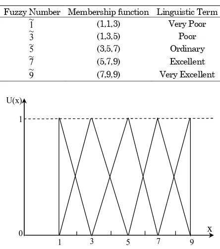
Fuzzy quantities are specifically represented with fuzzy numbers with interval between 0 and 1. A fuzzy quantity, M(x), is used to measure the proximity of M(x) predicting a real number r. In so doing, Triangular fuzzy numbers (TFNs) are easy and practical to use in a fuzzy environment. A triangular fuzzy number, M~is shown in Figure 1 [7].

The TFNs in a fuzzy event have three parameters: l, m, and u, indicating the smallest, the most pro-mising, and the largest possible values respectively. Their membership functions are defined as follows:

As the confidence interval level is expressed with , TFN is defined as:

Some positive fuzzy numbers main operations expressed with the confidence interval are:

] scales as shown in Tables 1 and 2 respectively.

~

Figure 1. A Triangular Fuzzy Number,M~

Table 1. Fuzzy Number, Membership function and

Linguistic Term

Fuzzy Number Membership function Linguistic Term

1

Figure 2. Triangular Fuzzy Ratio Scales

FAHP

A fuzzy ratio scale exactly corresponds to a sub score,G~_ijk,representing the sub-score of alternative,

Ai, with respect to sub-criterion, Cjk. After obtaining

all Gijk ~

of Ai with respect to all Cjk, the judgement

score,~a_ij,is computed. Equation 4 is used to

separa-tely aggregate all Ai, with respect to Cjk, which

All scores from Equation 1 are calculated to form a decision matrix. A normalisation process is conducted to allow a matching process with the weight vector. Each criterion, Cj, in a decision matrix

is normalised by using Equation 5. A fuzzy judge-ment matrix, A, is obtained after normalising.

ij fuzzy weight vector to obtain the fuzzy performance matrix, H. This represents the overall fuzzy performance which each alternative corresponds to all criteria. Meanwhile, the weight vector represents the relative importance among each criterion is

calculated with AHP PC or with immediate expert’s

(3)

The different experts may define the different weight vectors because they usually give the imprecise evaluation during the decision process. To handle this, a group of decisions on AHP with TFN are used to improve the original PC. A comprehensive PC matrix, D is constructed by integrating all decision

makers’ grades, bjep, through Equations 6 to 10. A

score bjep represents a decision maker Dp, measures of the relative importance by using Saaty’s scale 1-9 between each criteria.

Lje=min (bjep), p=1,2,…t j=1,2…m e=1,2….m (6)

importance among each criterion with TFN. In order to acquire a weight, w~_j, which corresponds to a

specific criterion, Cj, the relative weights between all

criteria is calculated as follows:

j weight vector, W, as in Equation 11.

W = (w~1,w~2,...w~m) (11) The experts’ subjective judgement produces uncer -tain and imprecise relations between criteria and alternatives and is usually accompanied with some

unclear factors including the decision maker’s degree

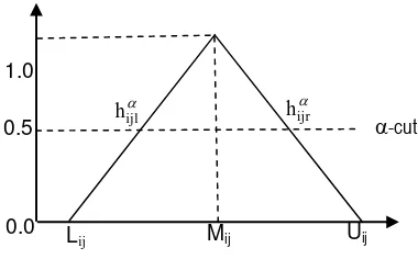
of confidence and degree of optimism of decision making. To overcome this situation, defuzzification is carried out by performing the interval performance matrix with -cut and the optimism index, . The

respectively represent

the left point and right point of the range of the triangle after using -cut. The range of is between 0 and 1. If the decision makers establish the higher degree of confidence, , it shows they have asked sufficient information to support their decisions. Therefore, the higher degree of confidence is corresponding to the lower uncertainty.



makers’ attitude that may be: optimistic, moderate,

or pessimistic. The optimism index is also applied to be a defuzzifier. Defuzzification is conducted by joining the optimism index to produce the final crisp numbers. The overall crisp performance matrix, H_

is calculated as follows [3]: 

 ij

h = h_ijl + (1- )h_ijr , 0 1 0 1 (14)

The h_ij_indicates the crisp performance score which

each alternative, Ai, corresponds to all criteria, Cj

under and .

TOPSIS

Technique for Order Preference by Similarity to Ideal Solution (TOPSIS) defines two kinds of solutions including the positive and negative ideal solutions. The positive ideal solution is the maximal benefits solution, and containing all best values of criteria. On the other hand, the negative ideal solution is the minimal benefits solution and composed of the all worst values of criteria. TOPSIS defines solutions as the points which are nearest to the positive ideal point and farthest from the

In which, J={j=1,2,…m| j belongs to positive criteria}

and J’={j=1,2,…m| j belongs to negative criteria}.

The distance between positive ideal solution and negative ideal solution for each alternative is respectively calculated as follows:

(4)

The Siand Si_{represent the distance between the} crisp performance scores of an alternative with respect to all criteria, all the positive and negative ideal solutions respectively. The relative closeness to the ideal solution for each alternative can be formulated using closeness coefficient, CC, as follows [7]:

 





 _

 



i i

S S

S

CC i = 1,2,…n (19)

The CCi indicates a final performance score

containing the decision maker’s degree of confi-dence about their valuations and degree of optimism. The larger final performance score expresses the more prior alternative.

Model Application and Results

Case Study Area and Data Descriptions

Total provincial roads lengths in Bali are 883.07 km [8]. These roads are distributed in eight regencies and one city in Bali. This study uses the same data employed in a previous study by Sutika [1]. Sutika [1] used macro transportation system to construct the main and sub criteria in determining provincial road handling in Bali. The system consists of three sub-systems; sub-system of activities (land use), movements (traffic flows), and network. These three sub-systems are related to each other and controlled by institutional sub-system [2].

In the land use sub-system, land will have a portion for certain activities. Meanwhile, movements are caused by the process of fulfilling needs, which cannot be met only at one type of land. Trips from one area to another will require transportation facilities including both mode of transport and infrastructures. Both are required to support the trips and are part of the network sub-system. Network sub-system facilitates a way for traffic movements so that its performance will be appro-priately measured by road surface conditions and road functions of the network itself. As the result, road surface conditions and road functions are used as the sub-criteria for the network sub-system.

With reference to the Bali Provincial Regulation No. 3 Year 2005 on Spatial Planning of Bali Province [9], land use in Bali Province is divided into two allotments; protected areas, and development area including office area, tourism, holy places, and mining. This division will be considered as a basis to form the sub-criteria of land use sub-system. For the institutional sub-system two approaches were considered to form its sub-criteria. They are top-down and bottom-up approaches. Top-top-down approach refers to the priority of local government policy on road handling while bottom-up approach provides significant space for community participations.

The data in Sutika [1] was collected through a questionnaire survey to obtain preferences amongst ten experts concerning Bali provincial road handling priority. Pairwise comparisons for each levelconsidering

Goal Criteria Sub Criteria Road Link (Number)

(D) Movements sub system (22%) (C) Land use sub system (11%)

(

(A) Institutional sub system (8%)

(B) Network sub system (59%)

Determining Provincial road

Handling Priority

(D1) Annual Daily Traffic (22%) (C4) Holy area and places

(2.20%) (C3) Mining area

(0.99%) (C1) Tourist and Nature Preserved

Area (5.94%)

(C2) Office area (1.87%) (A1) Top-down approach (5.5%)

(A2) Bottom up approach (2.5%)

(B1) Road conditions (45.43%)

(B2) Road function (13.57%)

025 053 030 0542 029 026 035 321 035

…. …. …. …. …. …. …. ….

06713 K 066 080 093 06712 K 06711 K 03812 K 05011 K 08011 K 08012 K 08013 K 08014 K 079 077 094

(5)

goal of these experts were carried out using a nine-point scale. Each pairwise comparison, PC was corresponded into an estimate of the priorities of the compared decision makers requirements [3].

The decision team making consisting ten experts of government officers, legislators, and academicians were involved in constructing these decision elements. The total number of alternatives con-sidered in the study were a hundred and forty road links. These were all provincial road links in Bali. As the results, all weight vectors of main and sub criteria were presented in Figure 4 [1]. Due to space limitation, however, Figure 4 only shows some road link numbers.

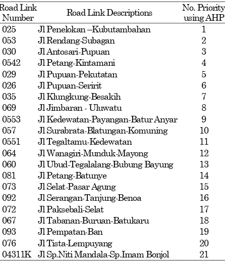
Sutika [1] used the secondary data of the Depart-ment of Public Works of Bali Province which provides the scores of all sub criteria for each alternative road link. This includes the scores of a hundred and forty road links under different road surface conditions. The judgements therefore, were conducted for each alternative (road link). Once the overall weight coefficient for each alternative is obtained, the highest weight coefficient value is taken as the best alternative. A very high priority scale is used to determine the priority for all provincial (140) road links in Bali. This scale is determined using AHP 0.85 percentile score or greater. As the results, there were twenty one road links that fall into this category as shown in Table 2 [1]. In other words, out of a hundred and forty provincial road links in Bali, twenty one road links were found with a very high priority for road handling.

Table 2. Road Handling Priority using AHP 0.85 Percen-tile [1]

Road Link

Number Road Link Descriptions

No. Priority using AHP

025 Jl Penelokan –Kubutambahan 1

053 Jl Rendang-Subagan 2

030 Jl Antosari-Pupuan 3

0542 Jl Petang-Kintamani 4

029 Jl Pupuan-Pekutatan 5

026 Jl Pupuan-Seririt 6

035 Jl Klungkung-Besakih 7

069 Jl Jimbaran - Uluwatu 8

0553 Jl Kedewatan-Payangan-Batur Anyar 9 057 Jl Surabrata-Blatungan-Komuning 10

0551 Jl Tegaltamu-Kedewatan 11

064 Jl Wanagiri-Munduk-Mayong 12

060 Jl Ubud-Tegalalang-Bubung Bayung 13

081 Jl Petang-Batunye 14

073 Jl Selat-Pasar Agung 15

092 Jl Serangan-Tanjung-Benoa 16

072 Jl Paksebali-Selat 17

067 Jl Tabanan-Buruan-Batukaru 18

093 Jl Pempatan-Ban 19

076 Jl Tista-Lempuyang 20

04311K Jl Sp.Niti Mandala-Sp.Imam Bonjol 21

Analysis and Results

An AHP’s crisp PC matrix used in the previous study

[1] is fuzzified using the TFN f = (l,m,u) as shown in Table 3. Both lower, l and upper, u, bounds present the uncertain range, that may occur within the

expert’s preferences. These TFNs are used to build

the comparison matrices (both the main and sub criteria) of FAHP based on pairwise comparison technique.

Table 3. Conversion of Crisp PCM – Fuzzy PCM [10] Crisp

PCM value

Fuzzy PCM value

Crisp PCM value

Fuzzy PCM value

1 (1,1,1) if diagonal (1,1,3) otherwise

1/1 (1/1,1/1,1/1) if diagonal (1/3,1/1,1/1) otherwise

2 (1,2,4) 1/2 (1/4,1/2,1/1)

3 (1,3,5) 1/3 (1/5,1/3,1/1)

5 (3,5,7) 1/5 (1/7,1/5,1/3)

7 (5,7,9) 1/7 (1/9,1/7,1/5)

9 (7,9,9) 1/9 (1/9,1/9,1/7)

A hierarchical structure for Bali provincial road handling priority problem is shown in Figure 4. The ultimate goal is located at level 1. At the next level, four major criteria are gathered so level 3 consisted of nine sub-criteria. Each road link is measured by all sub-criteria to obtain sub-scores. Each criterion respectively sums up its sub-scores. The sub scores of each road link with respect to all sub-criteria are obtained as shown in Table 4.

By Equation 4, all sub-scores of each road link are summed up with respect to the sub-criteria which belong to the same criterion to acquire all scores, G~_ij. The scores of each road link with respect to institutional subsystem, A, are calculated as:

11

~

G = G~₁₁₁ G~₁₁₂; G~₁₁= (7,9,9)(7,9,9) = (14,18,18) The rest may be calculated using the same way, so that the G matrix can be formed as shown in Table 5.

Road conditions with respect to each road link is normalised following Equation 5 as follows:

2 31 2 21 2 11

11

11 _~ _~ _~

~ ~

G G G

G a

 

 =

53.329) 44.000, (35.043,

(14,18,18)

= (0.263, 0.409, 0.514)

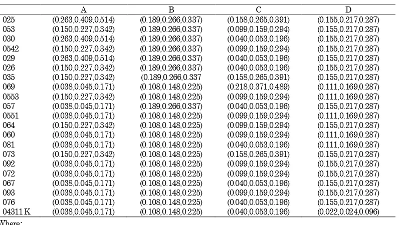
Using the same way, the fuzzy judgement matrix, A is constructed as shown in Table 6. A comprehensive pairwise comparison matrix, D, is calculated by

integrating the expert’s different opinions using

Equations 6 to 9. The D matrix is obtained as shown in Table 7. By using Equation 10, the fuzzy weight vector, W, is obtained as shown in Table 8.

(6)

Table 4. Scores of Each Road Link

A1 A2 B1 B2 C1 C2 C3 C4 D 025 ₉~ ~₉ ~₉ ₉~ ₉~ ~₁ ₁~ ₉~ ₉~ 053 ₁~ ~₉ ~₉ ₉~ 9 ~₁ ₁~ ₁~ ₉~ 030 ₉~ ~₉ ~₉ ₉~ ₁~ ~₁ ₁~ ₁~ ₉~ 0542 ₁~ ~₉ ~₉ ₉~ 9 ~₁ ₁~ ₁~ ₉~ 029 ₉~ ~₉ ~₉ ₉~ ₁~ ~₁ ₁~ ₁~ ₉~ 026 ₉~ ~₁ ~₉ ₉~ ₁~ ~₁ ₁~ ₁~ ₉~ 035 ₁~ ~₉ ~₉ ₉~ ₁~ ~₁ ₉~ ₉~ ₉~ 069 ₁~ ~₁ ~₉ ₁~ ₉~ ~₁ ₉~ ₉~ ₇~ 0553 ₁~ ~₉ ~₉ ₁~ ₉~ ~₁ ₁~ ₁~ ₇~ 057 ₁~ ~₁ ~₉ ₉~ ₁~ ~₁ ₁~ ₁~ ₉~ 0551 ₁~ ~₁ ~₉ ₁~ ₉~ ~₁ ₁~ ₁~ ₇~ 064 ₁~ ~₉ ~₉ ₁~ ₉~ ~₁ ₁~ ₁~ ₉~ 060 ₁~ ~₁ ~₉ ₁~ ₉~ ~₁ ₁~ ₁~ ₇~ 081 ₁~ ~₁ ~₉ ₁~ ₁~ ~₁ ₁~ ₁~ ₇~ 073 ₁~ ~₉ ~₉ ₁~ ₁~ ~₁ ₉~ ₉~ ₉~ 092 ₁~ ~₁ ~₉ ₁~ ₁~ ~₁ ₁~ ₉~ ₉~ 072 ₁~ ~₁ ~₉ ₁~ ₁~ ~₁ ₉~ ₁~ ₉~ 067 ₁~ ~₁ ~₉ ₁~ ₁~ ~₁ ₁~ ₁~ ₉~ 093 ₁~ ~₁ ~₉ ₁~ ₁~ ~₁ ₉~ ₁~ ₉~ 076 ₁~ ~₁ ~₉ ₁~ ₁~ ~₁ ₁~ ₁~ ₉~ 04311 K ₁~ ~₁ ~₁ ₉~ ₁~ ~₁ ₁~ ₁~ ₁~ Where:

A1 : Top down approach B2 : Road function C3 : Mining area A2 : Bottom up approach

C1 : Tourist and Nature Preserved Area C4 : Holly area and places

B1 : Road conditions C2 : Office area

D : Annual Daily Traffic

Table 5. All Scores, G Matrix

A B C D

025 (14,18,18) (14,18,18) (16,20,24) (7,9,9) 053 (8,10,12) (14,18,18) (10,12,18) (7,9,9) 030 (14,18,18) (14,18,18) (4,4,12) (7,9,9) 0542 (8,10,12) (14,18,18) (10,12,18) (7,9,9) 029 (14,18,18) (14,18,18) (4,4,12) (7,9,9) 026 (8,10,12) (14,18,18) (4,4,12) (7,9,9) 035 (8,10,12) (14,18,18) (16,20,24) (7,9,9) 069 (2,2,6) (8,10,12) (22,28,30) (5,7,9) 0553 (8,10,12) (8,10,12) (10,12,18) (5,7,9) 057 (2,2,6) (14,18,18) (4,4,12) (7,9,9) 0551 (2,2,6) (8,10,12) (10,12,18) (5,7,9) 064 (8,10,12) (8,10,12) (10,12,18) (7,9,9) 060 (2,2,6) (8,10,12) (10,12,18) (5,7,9) 081 (2,2,6) (8,10,12) (4,4,12) (5,7,9) 073 (8,10,12) (8,10,12) (16,20,24) (7,9,9) 092 (2,2,6) (8,10,12) (10,12,18) (7,9,9) 072 (2,2,6) (8,10,12) (10,12,18) (7,9,9) 067 (2,2,6) (8,10,12) (4,4,12) (7,9,9) 093 (2,2,6) (8,10,12) (10,12,18) (7,9,9) 076 (2,2,6) (8,10,12) (4,4,12) (7,9,9) 04311 K (2,2,6) (8,10,12) (4,4,12) (1,1,3)

Where:

A = Institutional sub-system B = Network sub-system C = Land Use sub-system D = Movements sub-system

During the priority ranking process, some unobvious factors which usually are ignored may deeply affect

the decision results. Therefore, the experts’ degree of

confidence and degree of optimism should be brought up during defuzzification process so that approaching the real decision. The value of 

indi-cates the experts’ degree of confidence in their

subjective evaluations concerning alternatives scores and criteria weight. The higher  value expresses the higher degree of confidence and closer to the possible value of the triangular fuzzy numbers. In addition, by using the  value (optimism index), defuzzification is conducted to obtain the crisp performance scores.

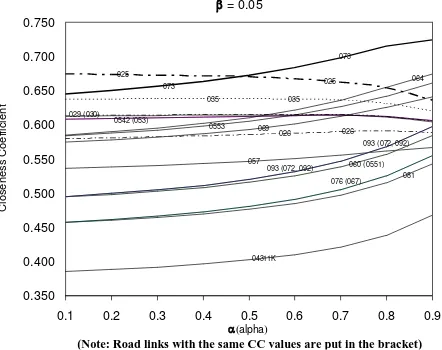
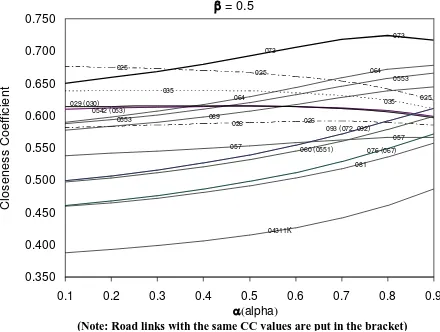
The crips performance scores and TOPSIS methods (Equations 14 to 18) are employed to determine the road link priority. The results which also showing the sensitivity analyses are depicted in Figures 5 to 7.These graphs show value as 0.05, 0.5 and 0.95 reflecting the pessimistic, the moderate, and the optimistics situations respectively. The horizontal and vertical axes showing the  varying from 0 to 1 and the closeness coefficient, CC values respectively.

The CC indicates the distance of road links from positive ideal solution in which the higher CC value expressing the higher priority. From the graphs, mutual comparisons can be performed from the most uncertain situation (=0) to the most certain situation (=1), from which the relative Bali provincial road link handling priority can be realised. Based on Figures 5 and 6, the Jl. Penelokan– Kubutambahan (025) is a road link with the highest priority in both pessimistic (=0.05) and moderate situations (=0.50) and from about certain ( 0.5) to the most uncertain conditions ( 0.35). Mean-while, Jl. Selat-Pasar Agung (073) is a road link with highest priority in such both situations and from about certain to the most certain conditions.

 = 0.05

025

0553

073 025

026 026 029 (030)

0542 (053)

035 035

069

057

064

060 (0551) 081 073

093 (072, 092)

093 (072, 092) 076 (067)

04311K

0.350 0.400 0.450 0.500 0.550 0.600 0.650 0.700 0.750

0.1 0.2 0.3 0.4 0.5 0.6 0.7 0.8 0.9

(alpha)

C

lo

se

n

e

ss

C

o

e

ff

ici

e

n

t

(Note: Road links with the same CC values are put in the bracket)

(7)

Table 6. Fuzzy Judgement Matrix

A B C D

025 (0.263,0.409,0.514) (0.189,0.266,0.337) (0.158,0.265,0.391) (0.155,0.217,0.287) 053 (0.150,0.227,0.342) (0.189,0.266,0.337) (0.099,0.159,0.294) (0.155,0.217,0.287) 030 (0.263,0.409,0.514) (0.189,0.266,0.337) (0.040,0.053,0.196) (0.155,0.217,0.287) 0542 (0.150,0.227,0.342) (0.189,0.266,0.337) (0.099,0.159,0.294) (0.155,0.217,0.287) 029 (0.263,0.409,0.514) (0.189,0.266,0.337) (0.040,0.053,0.196) (0.155,0.217,0.287) 026 (0.150,0.227,0.342) (0.189,0.266,0.337) (0.040,0.053,0.196) (0.155,0.217,0.287) 035 (0.150,0.227,0.342) (0.189,0.266,0.337 (0.158,0.265,0.391) (0.155,0.217,0.287) 069 (0.038,0.045,0.171) (0.108,0.148,0.225) (0.218,0.371,0.489) (0.111,0.169,0.287) 0553 (0.150,0.227,0.342) (0.108,0.148,0.225) (0.099,0.159,0.294) (0.111,0.169,0.287) 057 (0.038,0.045,0.171) (0.189,0.266,0.337) (0.040,0.053,0.196) (0.155,0.217,0.287) 0551 (0.038,0.045,0.171) (0.108,0.148,0.225) (0.099,0.159,0.294) (0.111,0.169,0.287) 064 (0.150,0.227,0.342) (0.108,0.148,0.225) (0.099,0.159,0.294) (0.155,0.217,0.287) 060 (0.038,0.045,0.171) (0.108,0.148,0.225) (0.099,0.159,0.294) (0.111,0.169,0.287) 081 (0.038,0.045,0.171) (0.108,0.148,0.225) (0.040,0.053,0.196) (0.111,0.169,0.287) 073 (0.150,0.227,0.342) (0.108,0.148,0.225) (0.158,0.265,0.391) (0.155,0.217,0.287) 092 (0.038,0.045,0.171) (0.108,0.148,0.225) (0.099,0.159,0.294) (0.155,0.217,0.287) 072 (0.038,0.045,0.171) (0.108,0.148,0.225) (0.099,0.159,0.294) (0.155,0.217,0.287) 067 (0.038,0.045,0.171) (0.108,0.148,0.225) (0.040,0.053,0.196) (0.155,0.217,0.287) 093 (0.038,0.045,0.171) (0.108,0.148,0.225) (0.099,0.159,0.294) (0.155,0.217,0.287) 076 (0.038,0.045,0.171) (0.108,0.148,0.225) (0.040,0.053,0.196) (0.155,0.217,0.287) 04311 K (0.038,0.045,0.171) (0.108,0.148,0.225) (0.040,0.053,0.196) (0.022,0.024,0.096) Where:

Table 7. Pairwise Comparison Matrix

A B C D

A (1.000,1.000,1.000) (0.111,0.513,3.000) (0.200,0.840,3.000) (0.200,0.613,3.000) B (0.333,6.133,9.000) (1.000,1.000,1.000) (1.000,4.800,7.000) (1.000,4.400,7.000) C (0.333,2.333,5.000) (0.143,0.282,1.000) (1.000,1.000,1.000) (0.200,0.507,1.000) D (0.333,3.333,5.000) (0.143,0.362,1.000) (1.000,2.800,5.000) (1.000,1.000,1.000) Where:

Table 8. Fuzzy Weight Vector

WA = (0.028, 0.096, 1.112) WB = (0.062, 0.528, 2.668) WC = (0.031, 0.133, 0.889) WD = (0.046, 0.242, 1.334)

Table 9.Fuzzy Performance Matrix

A B C D

025 (0.007,0.039,0.571) (0.012,0.140,0.900) (0.005,0.035,0.348) (0.007,0.053,0.383) 053 (0.004,0.022,0.381) (0.012,0.140,0.900) (0.003,0.021,0.261) (0.007,0.053,0.383) 030 (0.007,0.039,0.571) (0.012,0.140,0.900) (0.001,0.007,0.174) (0.007,0.053,0.383) 0542 (0.004,0.022,0.381) (0.012,0.140,0.900) (0.003,0.021,0.261) (0.007,0.053,0.383) 029 (0.007,0.039,0.571) (0.012,0.140,0.900) (0.001,0.007,0.174) (0.007,0.053,0.383) 026 (0.004,0.022,0.381) (0.012,0.140,0.900) (0.001,0.007,0.174) (0.007,0.053,0.383) 035 (0.004,0.022,0.381) (0.012,0.140,0.900) (0.005,0.035,0.348) (0.007,0.053,0.383) 069 (0.001,0.004,0.190) (0.007,0.078,0.600) (0.007,0.049,0.435) (0.005,0.041,0.383) 0553 (0.004,0.022,0.381) (0.007,0.078,0.600) (0.003,0.021,0.261) (0.005,0.041,0.383) 057 (0.001,0.004,0.190) (0.012,0.140,0.900) (0.001,0.007,0.174) (0.007,0.053,0.383) 0551 (0.001,0.004,0.190) (0.007,0.078,0.600) (0.003,0.021,0.261) (0.005,0.041,0.383) 064 (0.004,0.022,0.381) (0.007,0.078,0.600) (0.003,0.021,0.261) (0.007,0.053,0.383) 060 (0.001,0.004,0.190) (0.007,0.078,0.600) (0.003,0.021,0.261) (0.005,0.041,0.383) 081 (0.001,0.004,0.190) (0.007,0.078,0.600) (0.001,0.007,0.174) (0.005,0.041,0.383) 073 (0.004,0.022,0.381) (0.007,0.078,0.600) (0.005,0.035,0.348) (0.007,0.053,0.383) 092 (0.001,0.004,0.190) (0.007,0.078,0.600) (0.003,0.021,0.261) (0.007,0.053,0.383) 072 (0.001,0.004,0.190) (0.007,0.078,0.600) (0.003,0.021,0.261) (0.007,0.053,0.383) 067 (0.001,0.004,0.190) (0.007,0.078,0.600) (0.001,0.007,0.174) (0.007,0.053,0.383) 093 (0.001,0.004,0.190) (0.007,0.078,0.600) (0.003,0.021,0.261) (0.007,0.053,0.383) 076 (0.001,0.004,0.190) (0.007,0.078,0.600) (0.001,0.007,0.174) (0.007,0.053,0.383) 04311 K (0.001,0.004,0.190) (0.007,0.078,0.600) (0.001,0.007,0.174) (0.001,0.006,0.128)

Where:

(8)

 = 0.5

Figure 6. Sensitivity Analysis - Moderate Situation

 = 0.95

025

026 035 069 025

0542 (053) 029 (030) 026

Figure 7. Sensitivity Analysis-Highly Optimistic Situation

Figure 7 shows that Jl. Selat-Pasar Agung (073) is a road link with the highest priority in higly optimistic situation (= 0.95) and for all conditions. For pessimistic, moderate and optimistic situations and for all conditions ranging from under the most uncertain to certain comparisons, a road link connecting between Jl Sp.Niti Mandala-Sp.Imam Bonjol(04311K) has the lowest priority.

Apparently, Figures 5, 6, and 7 show 15 priority lines instead of 21 lines. This is because some road links have the same CC values. These similar road links numbers are put in the bracket.

Meanwhile, the ranking of road handling priority in the previous study using the AHP method for the same set of data is shown in Table 2 [1]. The table shows that Jl Penelokan–Kubutambahan (025) is a road link with the highest road handling priority. The current study results shows that Jl. Penelokan– Kubutambahan (025) is a road link with the highest priority in both pessimistic (=0.05) and moderate situations (=0.50) and from about certain ( 0.5) to the most uncertain conditions ( 0.35). This is shown in Figures 5 and 6. Meanwhile, both previous

and current studies suggest that Jl Sp.Niti Mandala-Sp.Imam Bonjol (04311K) has the lowest road handling priority.

The rest of the priority resulted from the current study, however is different to the previous study. The road handling priority resulted from this study however, is preferred in comparison to that of the previous study as the current study has also considered the decision maker’s degrees of confidence and optimism of the decision.

Conclusions

In this study, Fuzzy AHP -cut based and TOPSIS methods are employed to determine Bali provincial road handling priority.A very high priority scale is used to determine the priority for all provincial (140) road links in Bali. This scale is determined using AHP 0.85 percentile score or greater. As the results, there are twenty one road links that fall into this category. These road links are analysed using FAHP -cut based and TOPSIS methods to determine Bali provincial road handling priority.

The decision maker’s degree of optimism in Bali Province, however, may have considerable impact on decision making. Adoption of these FAHP -cut based and TOPSIS methods allow the researcher to estimate the overall road handling priority from optimistic to pessimistic and from under the most uncertain to certain comparisons.

The previous study results using the AHP method are compared to the current study for the same set of

data. The current study shows that decision makers’

degree of confidence in both pessimistic and moderate situations and optimism from about certain to the most uncertain conditions suggesting the same road link as the highest priority compared to the previous study. Both current and previous studies also conclude the same road link as the lowest road handling priority. The road handling priority resulted from this study, however, is preferred in comparison to that of the previous study as the current study has also considered the decision

maker’s degrees of confidence and optimism of

decision.

References

1. Sutika, I.K., Determining Provincial Road

Handling Priority in Badung Regency using AHP Method (in Indonesian), M.Eng Thesis, Post-graduate Programme in Civil Engineering, Udayana University, Bali, 2010.

(9)

3. Kwong, C.K. and Bai, H., A Fuzzy AHP Approach to the Determination of Importance Weights of Customer Requirements in Quality Function Deployment, Journal of Intelligent Manufac-turing, Vol. 13, 2002, pp. 367-377.

4. Saaty, T.L., Decision Making for Leaders: The Analytical Hierarchy Process for Decision in Complex World. Pittsburgh: University of Pitts-burgh, 1986.

5. Vahidnia, M.H., Alesheikh, A., Alimohammadi, A., and Bassiri, A., Fuzzy Analytical Hierarchy Process in GIS Application, The International Archives of the Photogrammetry, Remote Sensing and Spatial Information Sciences, Vol. XXXVII, Part B2, Beijing, 2008.

6. Dagdeviren, M., Yavuz, S., and Kılınç, N., Weapon selection using the AHP and TOPSIS Methods

under Fuzzy Environment, Expert Systems with Applications, Vol. 36, 2009, pp. 8143–8151.

7. Ballı, S. and Korukoğlu, S., Operating System Selection Using Fuzzy AHP and TOPSIS

Methods, Mathematical and Computational

Applications, Vol. 14, No.2, 2009, pp. 119-130.

8. Department of Public Works, 2009-2013 Strategic Planning. Department of Public Works of Pro-vince of Bali (in Indonesian), Bali, 2009.

9. Bali Provincial Government, Bali Provincial Regulation No. 3 2005: Spatial Planning of Bali Province 2005-2010 (in Indonesian), Bali, 2005.