and Education in Estimates of the
Conditional Wage Gap Between Black
and White Women
Peter McHenry
Melissa McInerney
McHenry and McInerneyA B S T R A C T
While evidence about discrimination in U.S. labor markets typically implies preferential treatment for whites, recent studies document a substantial wage premium for black women (for example, Fryer 2011). Although differential selection of black and white women into the labor market has been a suggested explanation, we demonstrate that accounting for selection does not eliminate the estimated premium. We then incorporate two additional omitted variables recently documented in the literature: (1) local cost of living and (2) years of education attained, conditional on AFQT score. After controlling for these variables, we fi nd no evidence of a wage premium for black women.
I. Introduction
Concerns about discrimination in labor markets have long motivated economists to compare labor market outcomes—wages in particular—between members of different groups. The history of race relations in the United States puts a focus on black- white differences, and many studies have found that black workers tend to earn lower wages than white workers with similar characteristics like age and education.1 More recently, however, several studies document higher wages among black—relative to white—women with similar characteristics (for example, Fryer 2011; Fisher and Houseworth 2012; Black et al. 2008). Such black wage premiums
1. See Lang and Lehmann (2012) for an excellent review.
Peter McHenry is an assistant professor of economics at the College of William and Mary. Melissa McInerney is an assistant professor of economics at the College of William and Mary. This research was conducted with restricted access to Bureau of Labor Statistics (BLS) data. For advice on acquiring the data, consult the authors beginning January 2015 through December 2017. The views expressed here do not necessarily refl ect the views of the BLS. They thank Sara Gault, Jason Saunders, and Xingchen Wang for excellent research assistance and three anonymous referees for excellent comments.
[Submitted February 2012; accepted June 2013]
ISSN 0022- 166X E- ISSN 1548- 8004 © 2014 by the Board of Regents of the University of Wisconsin System
The Journal of Human Resources 696
are puzzling in light of other fi ndings of discrimination against black workers (for example, Bertrand and Mullainathan 2004; Fryer, Pager, and Spenkuch 2011). 2
A common thread in the studies fi nding a black wage premium among women is to control for test scores (usually the AFQT) as a proxy for general academic ability and/or labor market productivity. For example, Fryer (in the 2011 Handbook of Labor Economics) fi nds that black women earn 12.7 percent more than otherwise similar white women (controlling for age, AFQT score, and its square). The magnitude of this estimated premium is striking, and Fryer (2011) cites selection into (or out of ) the labor force as a potential explanation. Whereas the performance of blacks relative to whites is likely overstated in estimates that do not control for selection, prior estimates of wage disparities that account for selection out of the labor force only reduce black wages (relative to white wages) by three to fi ve percentage points (for example, Neal 2004). We begin by demonstrating that accounting for selection out of the labor market is not suffi cient to eliminate the black wage premium in our sample of women in the 2006 National Longitudinal Survey of Youth 1979 (NLSY79).
We then turn to two important omitted variables: cost of living and years of educa-tion (see Black et al. 2012; Lang and Manove 2011). Omitting either variable from estimates of racial wage differences is likely to overstate black wages relative to white wages. We present a model of employer discrimination to show explicitly how racial wage gap estimates might attribute racial differences in local costs of living to unequal pay due to discrimination. (See the Appendix.) To the extent that black and white women face different local costs of living, estimates of raw wage differentials do not provide an adequate measure of labor market disadvantages faced by particular groups (see also Black et al. 2012; DuMond, Hirsch, and Macpherson 1999). Many wage gap studies do not control for differential costs of living (for example, Murnane, Willett, and Levy 1995; Neal and Johnson 1996; Black et al. 2008; Fryer 2011). We show that black women tend to face higher local costs of living (for example, in larger cities), so estimates of wage gaps that fail to account for this will overstate how blacks are per-forming, relative to whites. We show that including controls for local costs reduces the wage differential. We control for local costs of living using restricted- access geocoded data that are not generally available to researchers, and we demonstrate the sensitivity of our racial wage gap evidence to alternative proxies for local costs (for example, an urban indicator) that are available in most public- use microdata sets.
In addition, for a given score on the AFQT, blacks acquire more years of education (Lang and Manove 2011). Because additional years of education are rewarded in the labor market, omitting years of education in estimates of wage gaps that also control for AFQT score results in upward biased estimates of the wage gap. Similar to the Lang and Manove (2011) results for black men, after we account for AFQT score and education in wage regressions, the estimated black wage premium among women falls substantially. The combination of cost of living and education controls eliminates the black wage premium.
After accounting for selection and including these two important omitted variables, we fi nd no evidence of black wage premiums for women. We then test the data further by examining three settings in which we would be most likely to observe a black- wage premium, if it exists. First, in the previous literature, the most consistent evidence of a black wage premium is among highly educated women (for example, Fisher and Houseworth 2012; Black et al. 2008). We estimate wage gaps separately by education level and fi nd no evidence of black wage premiums, even among highly educated women. Second, we add controls for occupation to wage regressions. To the extent that occupational sorting differs by race due to discrimination against black women, wage gaps conditional on occupation understate discrimination against black women (Blau and Ferber 1987). Equivalently, black women’s conditional wages should be high relative to white women’s wages, but our estimates that control for occupation again show little signifi cant difference between black and white women’s conditional wages. Third, researchers typically control for age or potential experience, but workers with the same education and age may have very different work experience histories, which imply very different labor market productivities. Because, on average, white women have more years of work experience than black women, we expect blacks will appear to perform even better, relative to whites, when we control for actual labor market experience. However, when we control for actual labor market experience, we
fi nd no statistically signifi cant wage premium. These fi ndings provide further evidence of no wage premium for black women.
II. Related Literature
A. The Role of Selection Out of the Labor Market in Estimates of Racial Wage Differences
Fryer (2011) cites selection out of the labor force as a potential explanation for the esti-mated black wage premium among women (page 859). Wage gaps that are computed from observed wages by defi nition exclude nonworkers, yet nonworkers might be an important group to consider in computing black- white wage differentials, especially if there are racial differences in patterns of work. Failing to account for selection out of work would result in blacks appearing to perform better than whites if black women with low potential wages are more likely to select out of work than white women and if white women with high potential wages choose not to work more frequently than black women.3 Empirical evidence tends to confi rm these expectations (see, for ex-ample, Neal 2004; and for a similar approach to accounting for selection out of work by males, see Johnson, Kitamura, and Neal 2000; Chandra 1999; Chandra 2003).
Neal (2004) shows the importance of accounting for both types of selection out of work when estimating the wage gap for women. With 1990 data, he imputes a low po-tential wage for low- educated women who did not work, received no fi nancial support from a spouse, but received Aid to Families with Dependent Children, Supplemental Security Income (SSI), or Food Stamps between 1988 and 1992. Considering
The Journal of Human Resources 698
tion out of work for nonworkers with low potential wages increases the wage gap between 2.8 and 3.7 percentage points. Some women choose not to work even with a high potential wage.4 When Neal (2004) also considers selection out of work by this group, the gap increases another 1 to 1.2 percentage points. Following Neal (2004), we account for differential selection out of the labor force for women with high and low potential wages.
B. The Role of Cost of Living in Estimates of Racial Wage Differences
There are other omitted variables whose exclusion might also overstate black wages, relative to whites. Blacks are more likely than whites to live in urban areas5, and costs of living are higher in urban areas. (See, for example, Albouy 2009; Fitzpatrick and Thompson 2010.) When estimating racial wage differences, omitting controls for the local cost of living is likely to show that black workers’ wages are higher relative to whites. In the Appendix, we describe a model of employer discrimination and the identifi cation of the wage effect of discrimination against black workers. If black workers live in relatively high- cost areas, then the estimate of discrimination is downward- biased. Because blacks face higher costs of living, their relative purchasing power is overestimated when omitting cost of living controls. However, estimates of racial wage differences that control for cost of living quantify racial differences in the power to make purchases from wage income.
Black et al. (2012) argue that if preferences are homothetic, a Mincer wage regres-sion must include separate residential location intercepts plus the usual controls in order to identify racial differentials in ability to fi nance the same level of utility from labor earnings. Black et al. (2012) estimate wage regressions with fi xed effects for location (defi ned as a Metropolitan Statistical Area (MSA) or the balance of the state in nonmetro areas) and fi nd that relative to specifi cations without location controls, conditional relative black wages fall by between three and fi ve percentage points. In-stead of location fi xed effects, DuMond, Hirsch, and Macpherson (1999) control for an explicit MSA cost- of- living measure when they estimate black- white wage gaps for women using Current Population Survey data from 1985 to 1995. As expected, they demonstrate that wages of black women fall relative to white women after controlling for cost of living.6
C. The Role of Educational Attainment in Estimates of Racial Wage Differences
As Lang and Manove (2011) show, controlling for AFQT score in a wage regression without also including years of education is appropriate only if, conditional on AFQT score, blacks and whites attain the same level of education. The authors fi rst present a model of statistical discrimination and educational sorting that is consistent with
4. Neal (2004) imputes high potential wages for nonworking women who have at least a high school degree, receive no welfare benefi ts between 1988-92, and are married to a high-earning spouse (making at least the 90th or 75th percentile in the income distribution among men of his own race).
5. Using the 2005-2007 American Community Survey (ACS), we compute that 88.8 percent of blacks live in a metropolitan area, compared with 79.1 percent of whites.
blacks acquiring more years of education than whites, conditional on AFQT score.7 Consistent with the model, blacks in the NLSY79 obtain higher levels of education than whites, conditional on AFQT scores: Black men with AFQT scores in the middle of the distribution attain 1.2 more years of education than white men. The disparity in educational attainment is even starker for women: At all but the lowest levels of AFQT scores, black women attain 1.3 more years of education than white women.
Therefore, since wage returns to education are positive, omitting a control for years of education in estimates of racial wage differences is expected to bias the coeffi cient on “black” upward.8,9 Lang and Manove (2011) show that including both the AFQT score and educational attainment causes black males to perform between six and eight percentage points more poorly than white males, but they do not examine the impact of controlling for educational attainment on the wage gap for women. Since, con-ditional on AFQT score, black women acquire even more education, we expect the impact of including years of education to be even larger.
III. Data and Empirical Strategy
A. Estimating Strategy
We begin by replicating prior estimates of the black wage premium for women us-ing the 2006 NLSY79. This longitudinal survey of 12,686 individuals was designed to be nationally representative of individuals between the ages of 14 and 22 in the year 1979. Respondents were interviewed annually through 1994, at which point it switched to a biennial survey. The NLSY79 data include detailed information about hourly wages, labor force participation, educational attainment, and AFQT score. We acquired the restricted- use fi les so that we can identify respondents’ counties of resi-dence within the United States (to measure cost of living). To replicate estimates in Fryer (2011), we estimate the following equation:
(1) Ln(wagei)= ␣ + BLACKi+␥1AFQTi+␥2AFQTi2+␦1agei+␦2agei2+i
where the estimate for β represents the conditional racial wage difference. If β is positive, our estimates are consistent with black women receiving a wage premium.
We then examine the impact of accounting for selection. In recent work, the most common approach to address selection out of work is to impute a potential wage for the nonworkers in the sample, and estimate median regressions of wage differentials (for example, Johnson, Kitamura, and Neal 2000; Chandra 2003; Neal 2004). Re-searchers include nonworkers in the estimation sample based on the assumption that
7. Under the assumption that it is harder for employers to estimate the productivity of a black worker than a white worker, employers place more weight on educational attainment when evaluating black workers. Therefore, black workers invest more in education than white workers do, in order to signal their productivity. 8. One concern is that the relevant omitted variable is school quality and that educational attainment proxies for school quality. If blacks attend schools of lower quality, on average, then blacks may acquire more schooling to acquire the same skills. This is unlikely to be the case. Lang and Manove (2011) show that including a host of school characteristics associated with school quality does not substantially change relative educational attainment by race, conditional on AFQT.
The Journal of Human Resources 700
the imputed wage and the wage an individual could potentially earn (potential wage) fall on the same side of the conditional median. Under this assumption, estimates are consistent for the population median without being sensitive to the chosen imputed value.
We account for differential selection by imputing low and high potential wages. We impute a low potential wage of $1 for women who: (1) received any benefi ts from the Temporary Assistance for Needy Families (TANF), Supplemental Security Income (SSI), or Food Stamp programs between 2002 and 2006; (2) have a high school degree or less education; and (3) report no spousal income in the previous fi ve years. We adopt these strict criteria to reduce the chance of errors because systematically imput-ing erroneous low potential wages for women of one race would impact our estimate of racial wage differences. For example, improperly imputing low potential wages for white women would result in overstated black relative wages.
We impute a high potential wage for women who meet the following two criteria: (1) married to a high- earning spouse and (2) earned at least some college education. We defi ne “high- earning spouse” in two ways. In our more conservative estimate, a high- earning spouse has average annual earnings over the past fi ve years that place him at or above the 90th percentile for men of his race in the 2006 NLSY79. We then loosen this restriction somewhat to include women whose spouse earns above the 75th percentile for men of his race. Improperly imputing high potential wages for black (but not white) women would result in overstated black relative wages. These criteria for imputation help ensure that the imputed wages are on the same side of the median as the respondent’s potential wage; however, adhering to these criteria leaves several groups of nonworking women without imputed wages, such as highly educated, unem-ployed, single women.10 If our decision rule leaves more highly skilled white women without an imputed wage than similar black women, then we would overstate relative black wages. 11
We next add controls for local cost of living to our OLS and median regression estimates. To justify these controls, we demonstrate that black and white women face systematically different costs of living. We measure locations as commuting zones (CZs), which are collections of counties defi ned by the U.S. Department of Agriculture to have signifi cant economic integration, measured by journey- to- work links (Tolbert and Sizer 1996). In metropolitan areas, CZs and MSAs overlap signifi cantly. The real advantage of using CZs as a unit of geography is in rural areas. With CZs, we do not need to drop all non- MSA areas or pool them together within each state or Census region (two common methods). Pooling is costly, as rural areas within a state can vary considerably. Consider Colorado, where rural areas include tourist towns like Breckenridge and also the San Luis Valley. Average monthly rent for two and three bedroom dwellings is $1,110 in the counties around Breckenridge but $540 in the San Luis Valley (2005–2009 ACS).
Housing is the most important local price in consumers’ budgets, and we use it as one proxy for local costs of living. Banzhaf and Farooque (2012) compare
alterna-10. We include women who are temporarily unemployed in our main OLS sample if they were working and had an observed wage in 2004.
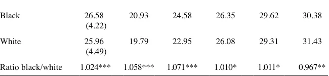
tive methods for measuring local housing costs and fi nd that average rental prices perform well: They are closely associated with housing transaction price data (which are more costly to collect), and rental prices are closely associated with measured local amenities and average incomes. Similar to Moretti (2013), we calculate average gross monthly rent (including utility costs) for two and three bedroom dwellings in each CZ with the pooled 2005 to 2007 ACS.12 In Table 1, Panel A we present the housing costs in CZs where the white and black women in the 2006 NLSY79 live. Column 1 shows blacks face higher costs of living on average: The black women in our sample face a mean monthly rent of $852 versus $816 for whites. The difference is statistically and economically signifi cant. The remaining columns of the table show that blacks face higher rent at several quantiles of the cost- of- living distribution.13
For the wage regressions, we construct a measure of relative housing costs for each CZ. We defi ne relative housing costs as the mean rent in a CZ divided by the average rent over all CZs. We use these relative housing costs to construct a cost of living index that refl ects that housing costs comprise only 42 percent of household expendi-tures (from the 2007 consumer price index (CPI- U) calculation).14
Of course, there are several concerns with rental costs as a measure of cost of living. For example, higher rental prices might be offset by lower costs of transportation or childcare for some individuals. If this is the case, rental prices do not accurately refl ect differences in the total cost of living. Relatedly, rental prices may be bid up by high- income households, but this does not correspondingly bid up prices for other goods.
Therefore, we also consider a second proxy for the cost of living that captures dif-ferences in wages across geographic areas. One concern with a wage- based measure of cost of living is that the higher wages paid in higher cost of living areas might
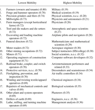
re-fl ect productivity differences among workers. Geographically mobile workers in par-ticular will live in areas with high productivity and wages. For this group of workers, the location- specifi c component of wages might refl ect unobserved individual produc-tivity. To mitigate such concerns, our wage- based measure of cost of living focuses on the wages of workers employed in occupations whose workers are relatively immo-bile geographically, such as farmers and funeral directors. (See Appendix Table A1.) A CZ’s average wage in these “low- mobility” occupations is our second control for
12. The smallest identifi able area in the ACS is the public use microdata area (PUMA), a Census-defi ned place with population over 100,000. Some PUMA boundaries do not perfectly align with counties. When this is the case, we assign PUMA characteristics to a CZ based on the PUMA’s population share in the CZ. (See McHenry 2014.)
13. Columns 2-6 describe the distribution of housing costs faced by NLSY79 black and white respondents. For example, Column 2 implies that 10 percent of black respondents to the NLSY79 live in CZs with average rental costs below $586 (as measured in the ACS), while 10 percent of white respondents live in CZs with average rental costs below $518.
14. That is, the CZ housing cost measure is computed as follows:
HousingCostCZ= MeanRentCZ
(
CZ=1
N
∑
MeanRentCZ)N
The Journal of Human Resources 702
Table 1
Local Cost of Living by Race, Characteristics of Locations Where NLSY79 Respondents Live
Percentile in the Distribution of NLSY79 Respondents’ Locations
Mean 10th 25th 50th 75th 90th
Panel 1: Average Rent for 2 to 3 Bedroom Property
Black 852.2
(246.0)
586.4 655.2 805.6 976.4 1,267
White 815.7
(245.4)
517.8 639.3 773.3 978.9 1,188
Ratio black/white 1.045*** 1.132*** 1.025** 1.042*** 0.997 1.066***
Panel 2: Mean Hourly Wage for Workers in “Low- Mobility” Occupations
Black 16.37
(1.86)
14.11 15.20 16.11 17.62 19.34
White 16.31
(1.97)
13.65 14.82 16.13 17.52 19.34
Ratio black/white 1.004 1.034*** 1.026*** 0.999 1.006 1.000
Panel 3: Mean Hourly Wage for Workers in “High- Mobility” Occupations
Black 26.58
(4.22)
20.93 24.58 26.35 29.62 30.38
White 25.96
(4.49)
19.79 22.95 26.08 29.31 31.43
Ratio black/white 1.024*** 1.058*** 1.071*** 1.010* 1.011* 0.967**
local costs of living.15 As shown in Table 1, Panel B, we fi nd that the average black woman lives in an area with higher wages among low- mobility occupations. The gap between local wages where black and white women live is highest in CZs at the lower end of the local wage distribution (that is, the 10th and 25th percentiles of respondents’ locations).16,17
In addition to cost of living, our preferred specifi cations control for years of educa-tion. If, conditional on AFQT score, black women acquire more years of education than white women, then omitting years of education would result in an upward bias on the coeffi cient estimate for the black indicator variable. Lang and Manove (2011) show that black women in the NLSY79 had acquired more years of education by 2000 than white women with the same AFQT score. We confi rm that this is true in 2006 as well.
Incorporating these methods, our preferred estimate of the black- white wage gap among women is the estimate for β in:
(2) Ln(wagei)= ␣ + BLACKi+␥1AFQTi+␥2AFQTi2+␦1agei+␦2agei2
+COLi+EDUCi+i.
This equation includes local cost of living (COL) and years of education (EDUC). The model of employer discrimination (in the Appendix) implies that local costs of living and individual productivity traits (like education) are important controls to in-clude; otherwise, the regression is unlikely to identify wage differences due to racial discrimination. We estimate Equation 2 using OLS and median regression. Observed log hourly wage among workers is the dependent variable for our OLS estimates. Median regression estimates also include nonworkers with imputed potential wages, described above.
B. NLSY79 Data
In Table 2, Columns 1 and 2, we present descriptive statistics for the black and white women in the sample we use for our OLS analysis. This sample includes women who worked and have valid wage information for either the 2006 or the 2004 survey. We
fi rst collect wage data from the 2006 survey but, for those missing wages in 2006, we use the 2004 wage if it is available. We convert wages to 2008 dollars using the
15. We identify noninstitutionalized workers ages 16-64 and employed in the private sector using the pooled 2005-2007 ACS at IPUMS (Ruggles et al. 2010). We collect residuals from a regression of log hourly wages on a quadratic in age and indicators for educational attainment, sex, and race/ethnicity. The average of those residuals among CZ residents employed in “low-mobility occupations” is our local wage index. An occupa-tion is considered “low-mobility” if more than half of the occupaoccupa-tion’s (3-digit OCC1990) workers were still living in their state of birth. An occupation is considered “high-mobility” if less than half of the occupation’s (three-digit OCC1990) workers were still living in their state of birth.
16. To address further concerns that the most productive workers choose to locate in the highest cost-of-living areas, we fi nd that although both of our cost-of-living measures are positively correlated with years of education and AFQT score, the magnitude is quite small. For example, increasing a respondent’s AFQT score from the 25th to the 75th percentile results in a 1.7 percent increase in the low-mobility occupation
wage measure.
704
Table 2
Descriptive Statistics from the NLSY79 (2006)
Sample: OLS Sample
(Columns 3–8: imputed wage)
15.66
(Columns 3–8: imputed wage)
12.87 15.40 1 1 45 45 45 45
Age at time of interview 44.67
(2.18)
Years of work experience at time of interview
CPI- U. When we compare unconditional mean and median hourly wages for the two groups, we see that white women earn more. For example, the mean hourly wage for white women is $19.31 and only $15.66 for black women: Blacks experience an unconditional wage penalty of 18.9 percentage points. Of course, comparing un-conditional means (or medians) does not take labor market skills into account. The bottom three rows of the table show that white women in the sample score higher on the AFQT, acquire 0.4 more years of education, and obtain nearly 2.5 more years of work experience.18
In Columns 3 and 4, we present descriptive statistics for the women who get a low imputed potential wage of $1, a group that includes twice as many black women as white women (84 versus 36). In Columns 5–8, we present summary statistics for the women who get a high imputed potential wage of $45. Both spousal earnings cutoffs imply high potential wage imputation for over four times as many white women as black women.
IV. Results
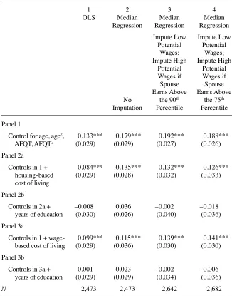
In Table 3, we present the coeffi cient estimate for β from Equation 1. In Column 1 of Panel 1, we confi rm Fryer’s (2011) result: Conditional on age and AFQT score, black women receive a wage premium of 0.133 log points (14.2 percent).19 The sharp contrast between this result and the 18.9 percent unconditional wage penalty
for black women (Table 2) is due to controlling for AFQT score, which is a proxy for academic ability and opportunities accumulated through age 18. Although there are im-portant racial disparities in opportunities before the age of 18, we begin our analysis of racial wage differences in the labor market by controlling for them with AFQT scores. Because outliers can infl uence OLS estimates, in Column 2 we present the median regression analog of Equation 1. The conditional wage premium in medians is even higher—0.179 log points. Of course, as Fryer (2011) notes, this estimate does not take into account selection out of the labor market. We account for selection in Columns 3 and 4, examining conditional median wages; therefore, it will be most appropriate to compare those results with the median regression output in Column 2.
In Column 3, we impute wage values for certain groups of nonworking women under the assumption that imputed wages fall either below or above the conditional median. We add 169 women to the sample with this addition. Seventy percent of the women with a low imputed wage are black and over 80 percent of women with a high imputed wage are white. Although these changes to the race- specifi c potential wage distributions would predict a decline in the estimated premium for black women, this only increases the sample size by nearly 7 percent. Thus, we fi nd no reduction of the black wage premium, as shown in Table 3, Column 3.20
18. Schooling and experience infl uence AFQT scores, so we normalize the raw AFQT score for each re-spondent by subtracting the mean score for others born the same year and dividing by the birth cohort’s standard deviation (similar to Neal and Johnson 1996).
19. We confi rmed that the slight difference from Fryer (2011) is due to his exclusion of individuals born before 1962 and his inclusion of Hispanics. Results are available upon request.
The Journal of Human Resources 706
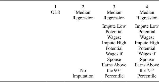
Table 3
Impact of Controls for Cost of Living and Educational Attainment on Estimates of Racial Differences in Hourly Wages for Women in 2006, Results from the NLSY79
1 2 3 4
Control for age, age2, 0.133*** 0.179*** 0.192*** 0.188***
AFQT, AFQT2 (0.029) (0.029) (0.027) (0.026)
Controls in 2a + –0.008 0.036 –0.002 –0.018
years of education (0.030) (0.026) (0.040) (0.036)
Panel 3a
Controls in 1 + wage- 0.099*** 0.115*** 0.139*** 0.141***
based cost of living (0.029) (0.036) (0.030) (0.030)
Panel 3b
Controls in 3a + 0.001 0.023 –0.002 –0.006
years of education (0.029) (0.029) (0.034) (0.036)
N 2,473 2,473 2,642 2,682
Notes: Dependent variable is the natural log of the hourly (or imputed) wage. Each regression includes age, age2, AFQT score and its square. In Column 1, heteroskedasticity robust standard errors are in parentheses.
In Column 4, we add to the sample 40 women without observed wages whose spousal earnings fall between the 75th and 89th percentiles in the distribution of earn-ings. We continue to fi nd a positive and statistically signifi cant black wage premium. Thus, we conclude that the black- wage premiums documented in the prior literature remain after accounting for selection. We now examine whether the estimated pre-mium is robust to including two important omitted variables: cost of living and years of education.
Subsequent rows of Table 3 present wage gap estimates that also control for the cost of living in an area and a respondent’s years of education. In Table 1, we showed that blacks live in CZs characterized by higher cost of living, whether we consider mean housing rents or higher wages paid to the least mobile occupations. We now present estimates that control for either of these two measures of cost of living. This is similar to the approach that DuMond, Hirsch, and Macpherson (1999) took for individuals residing in a MSA/CMSA. In Panel 2a of Table 3, we add a control for the average monthly rent in the CZ where the respondent lives. We fi nd that the black wage pre-mium estimate falls substantially in all specifi cations (Columns 1–4).
As Lang and Manove (2011) show, relative wages of black workers are overstated when we control for AFQT score but not years of education. In the third results row of Table 3, we control for years of education in addition to local costs of living. The additional control for education completely erases the estimated black wage premium. For the OLS results in Column 1, the coeffi cient on black turns slightly negative (a wage penalty), although the conditional racial wage gap is essentially zero. The same result holds in our median regression estimates that account for selection in Columns 3 and 4: Controls for cost of living and education (in addition to quadratics in age and AFQT score) yield no evidence of a black wage premium. We note that the 95 percent confi dence intervals for the conditional wage gap are somewhat large, and we are unable to reject substantial wage premiums (as high as 0.087, in Column 2) or wage penalties (as low as –0.089, in Column 4). Nevertheless, these specifi cations show clearly that the very large black wage premiums estimated in prior studies are not at all robust to reasonable controls for cost of living and education.
In Panels 3a and 3b of Table 3, we show that results are similar when we instead control for cost of living with a measure of average wages in “low- mobility” occupa-tions. Differential cost of living for black and white women explains away a large share (though not all) of the estimated black wage premium. When we also control for a respondent’s years of education, we again fi nd no evidence of a wage premium.21
A. Addressing Potential Concerns with Cost of Living Measures
A possible concern with our two cost of living measures is that we might not be cap-turing price differences across areas but are instead controlling for public sector em-ployment. This concern arises since blacks are more likely to work in the public sector than whites (U.S. Department of Labor 2012) and public sector jobs pay more (see, for example, Congressional Budget Offi ce 2012), especially in urban areas (Brueckner
observed in our sample ($156).
The Journal of Human Resources 708
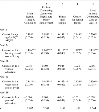
and Neumark 2011). In Table 4, Column 1 we replicate the coeffi cient estimates from Column 4 of Table 3, for comparison. In Column 2, we exclude respondents living in commuting zones where the share of public employees is above the 90th percentile (21.6 percent) and present the corresponding coeffi cient estimates. The same qualita-tive conclusion is upheld: The estimated wage premium disappears once we control for cost of living and education. Therefore, we do not believe that our measure merely proxies for public sector employment.
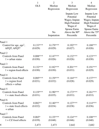
A second concern with the cost of living measure is that it might proxy for local school quality instead of local prices, because many of the areas with the highest cost of living have poorly performing public schools (for example, large cities). In response, we show that our main results hold when we also control for proxies of school quality (inputs to the respondents’ high school such as the share of teachers with higher degrees). These results are in Columns 3 and 4 of Table 4. In Column 3, we present results for the sample of respondents with valid school input measures as a baseline (note that this results in the loss of more than half the sample).22 In Column 4, we include school input variables and fi nd the same pattern as our main result: Controlling for cost of living and years of education erases the black- wage premium. Although we observe these measures of school quality, employers may not know the quality of schools for workers who have relocated since high school. Therefore, in Column 5 we restrict the sample to workers who lived in the same CZ in 2006 and age 14 since employers likely have a sense of school quality in their current location. Again, the qualitative conclusions are upheld, suggesting that our controls for cost of living are not merely picking up school quality.
B. Alternative Controls for Cost of Living
Our preferred way to account for workers’ locations is to control directly for local costs of living but doing so requires geocoded data that are often available only through restricted- use data licenses that are costly to obtain. For researchers estimat-ing wage gaps without such access, we examine the impact of usestimat-ing more widely available controls for region and urban status. In Panel 1 of Appendix Table A2, we show baseline log wage regressions that control for quadratics in age and AFQT. Panel 2 adds a control for urban status, which reduces the estimated black wage premium substantially.23 This is because the cost of living is higher in urban locations and black women are more likely to live in urban areas than white women. Adding region fi xed effects without an urban indicator (Panel 3) does not reduce the black wage premium (relative to Panel 1). This is because black women are more likely to live in the South, a region with lower costs of living. Including both a measure for urban status and
22. Even though the cost of living controls alone do not reduce the estimated premium in the school input re-sults shown, the main conclusion is upheld in this sample: Including controls for both cost of living and years of education eliminates the estimates of a wage premium. Furthermore, in results not shown we fi nd that in the sample of respondents with school input information, cost-of-living controls reduce the black wage pre-mium in every other specifi cation (that is, OLS, median regressions without imputations, and median regres-sions when we only impute high potential wages for women whose spouse earns above the 90th percentile).
Table 4
Median Regression Results from Different Samples, Impute Low Potential Wages and Impute High Potential Wages if Spousal Earnings Above the 75th Percentile
1 2 3 4 5
Control for age, 0.188*** 0.188*** 0.139*** 0.143** 0.206*** age2, AFQT,
AFQT2
(0.026) (0.029) (0.042) (0.061) (0.035)
Panel 2a
Controls in 1 + 0.126*** 0.142*** 0.112*** 0.119** 0.133***
housing- based cost of living
(0.033) (0.030) (0.040) (0.057) (0.036)
Panel 2b
Controls in 2a + –0.018 –0.005 –0.028 –0.028 –0.016
years of education
(0.036) (0.039) (0.051) (0.057) (0.044)
Panel 3a
Controls in 1 + 0.141*** 0.143*** 0.145*** 0.139** 0.139***
wage- based cost of living
(0.030) (0.031) (0.042) (0.058) (0.038)
Panel 3b
Controls in 3a + –0.006 0.001 –0.016 –0.021 –0.028
years of education
(0.036) (0.038) (0.051) (0.065) (0.050)
N 2,682 2,387 1,191 1,191 1,564
Notes: See notes to Table 3. In Column 2, we exclude commuting zones where the share of public employees is above the 90th percentile (21.6 percent). In Column 3, we preserve the individuals who have valid school
The Journal of Human Resources 710
region fi xed effects results in estimates of the black wage differential that are very similar to the corresponding results from Table 3 that control directly for local costs of living.24 We conclude that an indicator for urban status performs well as an alternative to direct cost of living controls in our context.
An alternative way of incorporating costs of living into a wage equation when geo-codes are available is to include fi xed effects that describe detailed locations. For example, Black et al. (2012) estimate wage regressions with a separate intercept for each location (defi ned as a Metropolitan Statistical Area or the balance of the state in nonmetro areas). When we include a separate intercept for each commuting zone (CZ) in Panel 7, we obtain similar results to our direct controls for cost of living. Neverthe-less, we believe that direct controls for cost of living are preferable when detailed geocode information is available. Because fi xed effects partial out all of the variation across cities (for example, Miami and Boston), and not just local prices, estimates of black- white wage gaps may be compromised if selective migration (for example, to large cities) makes up an important part of productivity (and wage) differentials between black and white workers. No matter which alternative cost of living measure we choose, we fi nd that once we control for years of education as well, the black wage premium is eliminated in most cases.
C. Testing for Presence of Black Wage Premium in Settings Most Likely to Show Premium
In the estimates presented thus far, we fi nd no statistically signifi cant evidence of a black wage premium, though we acknowledge that the standard errors are so large that we cannot rule out wage premiums as large as 0.087 log points (or wage penalties as low as –0.089 log points). To show more conclusively that we fi nd no evidence of a black wage premium once we control for cost of living and years of education, we now include these controls in subsamples and specifi cations that have traditionally shown black women performing the best relative to whites. If we continue to fi nd no evidence of a black wage premium in these settings, we can be even more confi dent that prior published estimates of statistically signifi cant black wage premiums were biased up-ward because they did not include controls for cost of living or years of education.
1. Racial wage differences among highly educated women
Several papers document a black wage premium among highly educated—or highly skilled—black women. (See, for example, Fisher and Houseworth 2012; Black et al. 2008.) Our results above might mask variation in the black- white wage gap across education groups. In Table 5, we separately examine racial wage differences for women with at least some college.25 For comparison purposes, we also present the racial wage differences for women with a high school degree or less.
When we control for AFQT, cost of living, and years of education, we fi nd no evidence of a wage premium among highly educated black women. This is especially
24. Panels 5 and 6 of Appendix Table A2 show that the inclusion of state fi xed effects also has only a modest impact on the black wage premium, much like region fi xed effects.
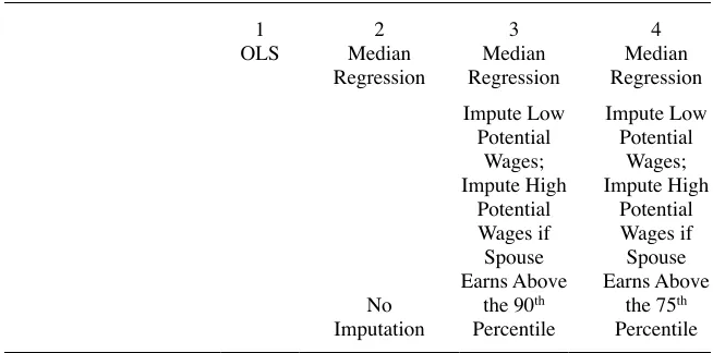
Table 5
Racial Differences in Hourly Wages for Women in 2006, by Education Level, Results from the NLSY79
1 2 3 4
OLS Median
Regression
Median Regression
Median Regression
No Imputation
Impute Low Potential
Wages; Impute High
Potential Wages if Spouse Earns Above
the 90th Percentile
Impute Low Potential
Wages; Impute High
Potential Wages if Spouse Earns Above
the 75th Percentile
Sample of Women with High School Degree or Less
Panel 1
Control for housing- –0.013 0.028 –0.014 –0.014
based cost of living (0.041) (0.048) (0.054) (0.054)
Panel 2
Control for wage- –0.007 0.015 0.007 0.007
based cost of living (0.041) (0.050) (0.051) (0.055)
N 1,152 1,152 1,272 1,272
Sample of Women with at Least Some College
Panel 3
Control for housing- –0.008 0.017 –0.007 –0.021
based cost of living (0.045) (0.042) (0.041) (0.046)
Panel 4
Control for wage- 0.004 0.038 0.003 –0.006
based cost of living (0.044) (0.044) (0.050) (0.047)
N 1,321 1,321 1,370 1,410
The Journal of Human Resources 712
notable since prior research has been most likely to fi nd a black wage premium in that group. In fact, if anything, relative wages for blacks are lower among the highly educated women than for the full sample. We note, however, that with the reduction of half of the sample size, these estimates are noisier than the full- sample estimates. Next, we turn to alternative specifi cations that preserve the full sample.
2. Role of controls for occupation and actual labor market experience
So far, we have not included controls for a worker’s occupation although the dis-tribution of workers across occupations infl uences racial wage differentials. If black women are systematically excluded from higher- paying occupations, then controls for occupation wipe out variation in wages that is caused by discrimination. Accord-ingly, wage gaps conditional on occupation have traditionally been interpreted as lower bounds for discrimination (Blau and Ferber 1987). However, recent evidence for males suggests that including controls for occupation might understate how well black women are performing relative to white women. Bjerk (2007) shows that, conditional on educational attainment, black (male) workers are more likely to choose to work in a white- collar occupation than a similar white (male) worker. Because white- collar occupations have higher average wages, adding a control for occupation to other premarket skills could reduce the estimate of black relative wages. We add controls for two- digit occupation to our preferred wage regression specifi cations and report the results in the fi rst two rows of Table 6 (separately for housing and wage- based controls).26 Even with occupation controls, there is little evidence of a statistically signifi cant black- wage premium among women. We document only one specifi cation that yields statistically signifi cant estimates: median regression estimates where we impute low potential wages and impute high potential wages for women whose spouse earns above the 75th percentile (t = 1.66).
Black women have signifi cantly fewer years of actual labor market experience rela-tive to whites. Therefore, comparing white and black women with the same potential
experience would tend to understate the human capital white women have developed. We expect that estimates of black- white wage differences that only include controls for a worker’s age or potential experience, such as the estimates described above in Tables 3 and 4, would result in blacks appearing to earn lower wages relative to whites. Antecol and Bedard (2002, 2004) show that since labor market attachment differs by race, actual experience explains much more of the wage gap than potential experience.27 Antecol and Bedard (2002) fi nd that length of work experience accounts for between 54–61 percent of the black- white wage gap among women.
Most estimates of racial wage differences do not include actual labor market ex-perience. This may be due to data availability or it may be because estimates of wage differentials often attempt to quantify discrimination, and differences in actual labor market experience may arise due to discrimination in hiring and retention. If
26. Some women with observed wages are missing occupation information. We create a category of missing occupation (but observed wages) for these women. We create two additional missing occupation categories: one for women with low imputed wages and one for women with high imputed wages.
Table 6
Impact of Occupation and Actual Work Experience Controls on Estimates of Racial Differences in Hourly Wages for Women in 2006
1 2 3 4
Control for housing- –0.001 0.023 0.034 0.034*
based cost of living (0.027) (0.029) (0.024) (0.020)
Panel 2
Control for wage- 0.010 0.035 0.035 0.030
based cost of living (0.027) (0.026) (0.023) (0.022)
N 2,473 2,473 2,642 2,682
Add Control for Actual Labor Market Experience
Panel 3
Control for housing- 0.006 0.030 0.019 0.010
based cost of living (0.027) (0.027) (0.030) (0.030)
Panel 4
Control for wage- 0.017 0.015 0.016 0.015
based cost of living (0.027) (0.032) (0.032) (0.027)
N 2,473 2,473 2,642 2,682
Notes: Regressions have the same form as Table 3 and Table 5: the dependent variable is the natural log of the hourly (or imputed) wage, and all specifi cations include controls for age, age2, AFQT score (and its square),
and years of schooling. Panels 1 and 2 add controls for two- digit occupation. For those missing occupation in either 2004 or 2006, we create three separate “missing occupation” categories. The fi rst category is for wage earners with no occupation. We create a second category for those with low imputed wages and a third category for respondents with high imputed wages. Panels 3 and 4 replace age (and age2) with years of actual
The Journal of Human Resources 714
minority women acquire lower levels of actual experience because they are the last hired and the fi rst fi red by discriminatory employers, then estimates of black- white wage differences that control for actual labor market experience do not capture the effect of this important discriminatory mechanism. For this reason, specifi cations that do not control for actual experience incorporate a potentially fuller picture of labor market discrimination and differential opportunities across groups. Nevertheless, we choose to examine estimates of racial wage differences that control for actual labor market experience because controls for actual labor market experience should in-crease relative wages of black workers and thereby make a black premium result more likely.
In the bottom panel of Table 6, we now include years of actual labor market experi-ence and its square. In every case, the coeffi cient estimate on “black” is positive and larger in magnitude than in regressions that instead controlled for a woman’s age; however, the estimates are never statistically signifi cant. Thus, even when we control for differences in human capital attributable to differences in hiring and retention, we fi nd no substantial evidence of black wage premiums. We interpret the estimates in Table 6 to be in the high range of likely relative wages of black women. Conse-quently, we argue that there is little evidence of a black wage premium among women overall.
V. Discussion
Prior work has shown that including either cost of living or education has an important impact on estimates of male wage gaps (Black et al. 2012; Lang and Manove 2011), and we have shown the importance of including both variables in estimates of wage gaps for black women. In Appendix Table A3, we now examine the impact of including both of these important variables in estimates of wage gaps for men (in the NLSY79 sample).28 In Column 1, we reproduce our OLS estimates for women. We note that including both controls reduces the coeffi cient on black by roughly 14 percentage points for women and approximately 11.8 percentage points for men (in Column 2). We note that the impact of including a control for cost of living is rather similar in the two samples, and that the real difference is observed with the additional control for years of education. Including a control for years of education reduces the coeffi cient on black by approximately nine percentage points for women and only nearly seven percentage points for men. This is not surprising because, as we noted above, conditional on AFQT score, racial differences in educational attainment are larger for women than for men.
Among men, we fi nd large conditional wage penalties associated with being black. In contrast, we fi nd no similar penalty for black women. For both men and women, however, wages of black—relative to white—workers are overstated in specifi cations that omit controls for cost of living or education.
VI. Conclusion
We fi nd no evidence of widespread wage premiums for black women
in our analysis of all black and white women once we account for selection out of the labor market, cost of living in one’s residential location, and educational attainment. Contrary to the hypothesis proposed in the literature, we fi nd no evidence that account-ing for selection explains away the wage premium. Instead, we fi nd these estimated wage premiums are sensitive to controls for residential location and educational attain-ment. We also show that incorporating these controls has a larger impact on estimates of wage gaps for women than for men. This is not surprising because, although black men and women both live in areas with relatively high costs of living, racial differ-ences in educational attainment—conditional on AFQT score—are larger for women than for men. That is, for a given AFQT score, blacks acquire more years of education than whites, and this gap is larger for women than for men.
One strand of the literature documents wage premiums for black relative to white women in samples of women with high levels of education. When we examine ra-cial wage differences among highly educated women, we fi nd no evidence of a wage premium. We then broaden the question we ask of our data and include controls for occupation or actual labor market experience (rather than age or potential experience). By wiping out potentially discriminatory variation in wages (through occupational segregation, hiring, and fi ring), both specifi cations yield estimates that are likely to be in the high range of black relative wages. However, even these estimates are smaller in magnitude than the wage premiums reported in the literature, and they provide little evidence consistent with a black wage premium.
The Journal of Human Resources 716
Appendix 1
Table A1
Occupations with the Lowest and Highest Shares of Workers Still Residing in Their Birth States
Lowest Mobility Highest Mobility
1. Farmers (owners and tenants) (0.80) Military (0.19)
2. Forge and hammer operators (0.78) Medical scientists (0.19) 3. Precision grinders and fi lers (0.74) Physical scientists, n.e.c. (0.20)
4. Millwrights (0.73) Physicists and astronomers (0.21)
5. Farm managers (except horticultural farms) (0.72)
Physicians (0.26)
6. Tool and die makers and die setters (0.72)
Atmospheric and space scientists (0.27)
7. Excavating and loading machine operators (0.72)
Airplane pilots and navigators (0.28)
8. Funeral directors (0.72) Mathematicians and mathematical
scientists (0.29)
9 Meter readers (0.72) Aerospace engineer (0.30)
10. Other mining occupations (0.72) Subject instructors (HS/college) (0.30)
11. Miners (0.71) Social scientists, n.e.c. (0.32)
12. Operating engineers of construction equipment (0.71)
Computer software developers (0.32)
13. Railroad brake, coupler, and switch operators (0.70)
Art/entertainment performers and related (0.33)
14. Protective services, n.e.c. (0.70) Dressmakers and seamstresses (0.34) 15. Firefi ghting, prevention, and
inspection (0.70)
Air traffi c controllers (0.34) 16. Winding and twisting textile/apparel
operatives (0.69)
Chemical engineers (0.34)
17. Repairers of mechanical controls and valves (0.69)
Biological scientists (0.35)
18. Other plant and system operators (0.69)
Plasterers (0.35)
19. Drillers of earth (0.69) Engineers, n.e.c. (0.36)
20. Lathe, milling, and turning machine operators (0.69)
Management analysts (0.36)
Appendix 2
Table A2
Using Fixed Effects to Control for Cost of Living
1 2 3 4
Control for age, age2, 0.133*** 0.179*** 0.192*** 0.188***
AFQT, AFQT2 (0.029) (0.029) (0.027) (0.026)
Panel 2
Controls from Panel 0.088*** 0.147*** 0.132*** 0.123***
1 + urban status (0.030) (0.026) (0.026) (0.030)
Panel 3
Controls from Panel 0.132*** 0.182*** 0.201*** 0.191***
1 + region fi xed effects (0.030) (0.030) (0.033) (0.029)
Panel 4
Controls from Panel 0.085*** 0.139*** 0.144*** 0.137***
1 + region fi xed effects + urban
(0.031) (0.032) (0.028) (0.029)
Panel 5
Controls from Panel 0.119*** 0.190*** 0.173*** 0.161***
1 + state fi xed effects (0.031) (0.035) (0.033) (0.033)
Panel 6
Controls from Panel 0.082** 0.140*** 0.127*** 0.114***
1 + state fi xed effects + urban
(0.032) (0.034) (0.038) (0.036)
Panel 7
Controls from Panel 0.065* 0.135*** 0.124*** 0.108***
1 + CZ fi xed effects (0.039) (0.048) (0.046) (0.040)
N 2,473 2,473 2,642 2,682
Notes: Regressions have the same form as Table 3: The dependent variable is the natural log of the hourly (or im-puted) wage, and all specifi cations include controls for age, age2, and AFQT score (and its square). Panels 2–7 add
The Journal of Human Resources 718
Appendix 3
Appendix 4
A Model of Employer Discrimination, Wage Gaps, and
Cost of Living
This section presents a simple economic model of racial discrimina-tion, wage gaps, and cost of living differences. The purpose of the model is to illustrate how discriminatory racial preferences of employers might be identifi ed with wage gaps when costs of living vary across locations. We note in particular the strong as-sumptions used to argue for such identifi cation.
The exposition and notation borrow heavily from Becker (1971) and Laing (2011). There is a representative fi rm owner in each location j who derives utility from profi t but disutility from paying black workers. That is, utility is increasing in revenues but
Table A3
Gender Differences in Importance of Controls for Cost of Living and Educational Attainment, OLS, Coeffi cient on Black
1 2
Women Men
Panel 1
Control for age, age2, AFQT, AFQT2 0.133*** –0.089***
(0.029) (0.031)
Panel 2a
Controls from panel 1 + housing- based 0.084*** –0.139***
cost of living (0.029) (0.030)
Panel 2b
Controls from panel 2a + years of education –0.008 –0.207***
(0.030) (0.030)
Panel 3a
Controls from panel 1 + wage- based cost 0.099*** –0.133***
of living (0.029) (0.030)
Panel 3b
Controls from panel 3a + years of education 0.001 –0.203***
(0.029) (0.030)
N 2,473 2,444
Notes: Dependent variable is the natural log of the hourly wage. Each regression includes age, age2, AFQT
decreasing in wages paid to all workers, and there is a further cost to utility from pay-ments to black workers, as shown in Equation A1, below. Workers vary based on their education, experience, and potentially other characteristics, and their types are indexed by i. The fi rm owner in location j has the utility function:
(A1) Uj= pjyj−
i
∑
wij Nij−i
∑
wijbNijb(1+␦)where pj is the price of output, yj is output, wij is the wage paid to white workers of type i in location j, Nij is the number of white employees of type i in location j, wijb and Nijb are corresponding wages and numbers of black workers, and ␦ is a preference pa-rameter, or the coeffi cient of employer discrimination. Higher values of ␦ imply greater racial animus toward black employees. Whereas quantities and prices may vary across locations j, we assume that racial animus measured by ␦ does not.
Worker types have different marginal productivities that do not vary by race or location and are defi ned by
MPi= MPexp
(
xi)
εiwhere MP is a baseline marginal productivity,  is a vector of parameters (skill prices), xi is a vector of such personal characteristics as education, and εi is an unobserved term that augments labor productivity. Assume that the fi rm owner takes wages as given and chooses the numbers of white and black workers to employ. Then, utility- maximizing hiring behavior implies that
wij= pjMPexp(xi)εi
and
wijb= pjMPexp(xi)εi/ (1+␦)
for each location j and worker type i. Taking logs of the previous equations implies
lnwij=lnpj+lnMP+xi+lnεi
and
lnwijb=lnpj+lnMP+xi+lnεi−ln(1+␦).
Researchers typically estimate residual racial wage gaps by regressing log wages on a constant (to estimate lnMP), the vector xi, and an indicator for race. The estimated residual racial wage gap is (letting Iij be an indicator variable for person i living in location j)29
␥b= 1
Nbiis
∑
black∑
jIijlnpj− 1 N
iis
∑
white∑
jIijlnpj+ 1 Nbiis
∑
blacklnεi
− 1
N
iis
∑
whitelnεi−ln 1
(
+␦)
.The Journal of Human Resources 720
Researchers may assume that unobserved determinants of wages in εi (for example, ability) are the same between black and white workers so
(A2) 1
Nbiis
∑
black lnεi− 1N
iis
∑
whitelnεi=0.
If it were also true that local prices faced by black and white workers were the same (that is, (Nb)−1⌺iisblack⌺jIijlnpj=(N)−1⌺iiswhite⌺jIijlnpj), then the coeffi cient on the black indicator would equal −ln(1+␦), allowing the identifi cation of employer animus toward black workers.
More generally though, omitting explicit controls for prices in a locality (lnpj) will bias estimates of the residual wage gap. For example, suppose blacks live in areas with higher prices (and higher costs of living) than whites (that is,
1 /Nb⌺iisblack⌺jIijlnpj>1 /N⌺iiswhite⌺jIijlnpj). If we fail to control for cost of living in the wage regression, then the estimated coeffi cient on the black indicator will attribute relatively high wages of blacks to the absence of discrimination rather than compensation for higher costs of living. The result would be an underestimate of dis-crimination (inferring a value of ␦ that is smaller than the true value).
In conclusion, wage regressions that include controls for local output prices and worker characteristics can identify the employers’ racial preference parameter ( ␦). We note, however, that such identifi cation relies on the very strong assumption in Equa-tion A2.
References
Albouy, David. 2009. “The Unequal Geographic Burden of Federal Taxation.” Journal of Political Economy 117(4):635–67.
Antecol, Heather, and Kelly Bedard. 2002. “The Relative Earnings of Young Mexican, Black, and White Women.” Industrial and Labor Relations Review 56(1):122–35.
———. 2004. “The Racial Wage Gap: The Importance of Labor Force Attachment Differences Across Black, Mexican, and White Men.” Journal of Human Resources 39(2):564–83. Banzhaf, H. Spencer, and Omar Farooque. 2012. “Interjurisdictional Housing Prices and
Spatial Amenities: Which Measures of Housing Prices Refl ect Local Public Goods?” NBER Working Paper #17809.
Becker, Gary S. 1971. The Economics of Discrimination, 2nd ed. Chicago: University of Chicago Press.
Bertrand, Marianne, and Sendhil Mullainathan. 2004. “Are Emily and Greg More Employable Than Lakisha and Jamal? A Field Experiment on Labor Market Discrimination.” American Economic Review 94(4):991–1013.
Bjerk, David. 2007. “The Differing Nature of Black- White Wage Inequality Across Occupa-tional Sectors.” Journal of Human Resources 42(2):398–434.
Black, Dan A., Amelia M. Haviland, Seth G. Sanders, and Lowell J. Taylor. 2008. “Gender Wage Disparities Among the Highly Educated.” Journal of Human Resources 43(3):630–59. Black, Dan A., Natalia Kolesnikova, Seth G. Sanders, and Lowell J. Taylor. 2012. “The Role
of Location in Evaluating Racial Wage Disparity.” Federal Reserve Bank of St. Louis Work-ing Paper #2009–043C.
Brueckner, Jan K., and David Neumark. 2011. “Beaches, Sunshine, and Public- Sector Pay: Theory and Evidence on Amenities and Rent Extraction by Government Workers.” NBER Working Paper #16797.
Bureau of Labor Statistics. 2007. “The Consumer Price Index.” In Handbook of Methods. Washington, D.C.: U.S. Department of Labor. www.bls.gov/opub/hom/pdf/ homch17.pdf.
———. 2013. “The Employment Situation – April 2013.” Washington, D.C.: U.S. Department of Labor.
Chandra, Amitabh. 1999. “Labor- Market Dropouts and the Racial Wage Gap: 1940–1990.” American Economic Review 90(2):333–38.
———. 2003. “Is the Convergence of the Racial Wage Gap Illusory?” NBER Working Paper Number 9476.
Congressional Budget Offi ce. 2012. “Comparing the Compensation of Federal and
Private- Sector Employees.” Washington, D.C.: Congress of the United States. www.cbo.gov/ sites/default/fi les/cbofi les/attachments/01- 30- FedPay.pdf
DuMond, J. Michael, Barry T. Hirsch, and David A. Macpherson. 1999. “Wage Differentials Across Labor Markets and Workers: Does Cost of Living Matter?” Economic Inquiry 37(4):577–98.
Fitzpatrick, Katie, and Jeffrey P. Thompson. 2010. “The Interaction of Metropolitan Cost- of- Living and the Federal Earned Income Tax Credit: One Size Fits All?” National Tax Journal 63(3):419–46.
Fisher, Jonathan D., and Christina A. Houseworth. 2012. “The Reverse Wage Gap Among Educated White and Black Women.” Journal of Economic Inequality 10(4):449–70. Fryer, Jr., Roland G. 2011. “Racial Inequality in the 21st Century: The Declining Signifi cance
of Discrimination.” In Handbook of Labor Economics, Volume 4b, ed. David Card and Orley Ashenfelter, 855–971. Amsterdam: Elsevier.
Fryer, Jr., Roland G., Devah Pager, and Joerg L. Spenkuch. 2011. “Racial Disparities in Job Finding and Offered Wages.” NBER Working Paper #17462.
Johnson, William, Yuichi Kitamura, and Derek Neal. 2000. “Evaluating a Simple Method for Estimating Black- White Gaps in Median Wages.” American Economic Review 90(2): 339–43.
Laing, Derek. 2011. Labor Economics: Introduction to Classic and the New Labor Economics. New York: WW Norton.
Lang, Kevin, and Jee- Yeon K. Lehmann. 2012. “Racial Discrimination in the Labor Market: Theory and Empirics.” Journal of Economic Literature 50(4):959–1006.
Lang, Kevin, and Michael Manove. 2011. “Education and Labor Market Discrimination.” American Economic Review 101(4):1467–96.
McHenry, Peter. 2014. “The Geographic Distribution of Human Capital: Measurement of Contributing Mechanisms.” Journal of Regional Science 54(2): 215–248.
Moretti, Enrico. 2013. “Real Wage Inequality.” American Economic Journal: Applied Econom-ics 5(1):65–103.
Murnane, Richard J., John B. Willett, and Frank Levy. 1995. “The Growing Importance of Cognitive Skills in Wage Determination.” Review of Economics and Statistics 77(2):251–66.
Neal, Derek. 2004. “The Measured Black- White Gap Among Women Is Too Small.” Journal of Political Economy 112(1):S1- S28.
Neal, Derek A., and William R. Johnson. 1996. “The Role of Premarket Factors in Black- White Wage Differences.” Journal of Political Economy 104(5):869–95.
The Journal of Human Resources 722
Ruggles, Steven, J. Trent Alexander, Katie Genadek, Ronald Goeken, Matthew B. Schroeder, and Matthew Sobek. 2010. Integrated Public Use Microdata Series: Version 5.0 [Machine- readable database]. Minneapolis: University of Minnesota.
Tolbert, Charles M., and Molly Sizer. 1996. “U.S. Commuting Zones and Labor Market Areas: A 1990 Update.” Rural Economy Division, Economic Research Service, U.S. Department of Agriculture. Staff Paper AGES- 9614.