Audrey Light is a professor of economics at Ohio State University. Andrew McGee is an assistant professor of economics at Simon Fraser University and a research fellow at IZA. The data used in this article can be obtained beginning June 2015 through May 2018 from Audrey Light, Department of Economics, Ohio State University, 410 Arps Hall, 1945 N. High Street, Columbus, OH 43210; email: light.20@osu.edu.
[Submitted March 2013; accepted January 2014]
ISSN 0022- 166X E- ISSN 1548- 8004 © 2015 by the Board of Regents of the University of Wisconsin System
T H E J O U R N A L O F H U M A N R E S O U R C E S • 50 • 1
“Importance” of Skills
Audrey Light
Andrew McGee
Light and McGeeabstract
We ask whether employer learning in the wage- setting process depends on skill type and skill importance to productivity, using measures of seven premarket skills and data for each skill’s importance to occupation- specifi c productivity. Before incorporating importance measures, we fi nd evidence of employer learning for each skill type, for college and high school graduates, and for blue- and white- collar workers, but no evidence that employer learning varies signifi cantly across skill or worker type. When we allow parameters identifying employer learning and screening to vary by skill importance, we identify tradeoffs between learning and screening for some (but not all) skills.
I. Introduction
learning, and by Bauer and Haisken- DeNew (2001), Arcidiacono, Bayer, and Hizmo (2010), and Mansour (2012) to investigate differences in employer learning across schooling levels, occupational type (blue- versus white- collar) and initial occupations, respectively.
In the current study, we ask whether the role of employer learning in the wage- setting process depends on the type of skill potentially being learned over time as well as the skill’s importance, by which we mean its occupation- specifi c contribution to productivity. Basic language skills might be readily signaled to potential employers via the job interview process while other skill types such as “coding speed” (the ability to fi nd patterns of numbers quickly and accurately) might only be revealed over time in the absence of job applicant testing. Moreover, a skill’s importance is likely to affect both ex ante screening technologies and the extent to which employers learn about the skill over time. If the ability to solve arithmetic problems is irrelevant to the work performed by dancers and truck drivers, for example, then the true productivity their employers learn over time should be uncorrelated with a measure of arithmetic skill. Stated differently, the relationship between arithmetic test scores and wages should not increase with experience for dancers and truck drivers. In reverse situations where a particular skill is essential to job performance, it is unclear whether signaling or learn-ing will dominate the wage- settlearn-ing process. Given that arithmetic skill is critical to accountants’ job performance, for example, should we expect arithmetic ability to be a key component of what their employers learn over time? Or do employers customize their screening methods to ensure that the most critical skills are accurately assessed ex ante?
To address these questions, we begin by identifying the channels through which skill importance enters a standard model of public employer learning. Using the omitted vari-able bias strategy of Altonji and Pierret (2001), we demonstrate that by using the portion of a test score (referred to as Z*) that is orthogonal to schooling and other regressors,
the Z*- experience gradient in a log- wage model is expected to depend solely on the test
score’s correlation with performance signals that lead to learning, while the coeffi cient for Z* is expected to depend both on skill importance and the extent to which the skill
is signaled ex ante. These derivations motivate our empirical strategy: First, we empiri-cally assess the role of employer learning for alternative skills by inserting skill- specifi c test scores (Z*) into a log- wage model and comparing the magnitudes of their estimated
experience gradients. Second, we allow coeffi cients for Z*and Z*- experience interactions
to depend on skill importance (which we measure directly) to determine whether learn-ing and screenlearn-ing depend on the skill’s importance to productivity.
We implement these extensions of the Altonji and Pierret (2001) model using data from the 1979 National Longitudinal Survey of Youth (NLSY79) combined with Oc-cupational Information Network (O*NET) data. To proxy for premarket skills that are unobserved by employers, we use test scores for seven components of the Armed Ser-vices Vocational Aptitude Battery (ASVAB). The use of narrowly defi ned test scores distinguishes our approach from the existing literature, where most analysts rely on scores for the Armed Forces Qualifi cations Test (AFQT)—a composite score based on four ASVAB components that we use individually.1 By using skill- specifi c test scores,
we can determine whether employer learning plays a different role for arithmetic abil-ity, reading abilabil-ity, coding speed, and so forth. We further extend the analysis by using O*NET data to measure the importance of each skill in the three- digit occupation associated with each job. These additional variables enable us to determine whether skill- specifi c screening and skill- specifi c employer learning are themselves functions of skill importance.
By allowing employer learning to vary with skill type and skill importance, we contribute to an emerging literature that explores heterogeneity in employer learn-ing along various dimensions. Bauer and Haisken- DeNew (2001) fi nd evidence of employer learning for men in low- wage, blue- collar jobs but not for other male work-ers; Arcidiacono, Bayer, and Hizmo (2010) fi nd evidence of employer learning for men with 12 years of schooling but not for men with 16 years of schooling; Mansour (2012) fi nds that employer learning differs across workers’ initial, two- digit occupa-tions. Our approach incorporates three innovaoccupa-tions. First, we allow for a richer form of heterogeneity than is permitted with a high school/college or blue- collar/white- collar dichotomy and, in fact, we demonstrate that employer learning does not differ across categories used by Bauer and Haisken- DeNew (2001) and Arcidiacono, Bayer, and Hizmo (2010). Second, while we incorporate Mansour’s (2012) notion that detailed measures of “job type” are needed to capture true heterogeneity in employer learning, we defi ne “job type” in terms of the skills needed to perform a specifi c task rather than occupational categories. We do so in light of existing evidence that jobs are better de-scribed in terms of tasks or skills than by orthodox occupational taxonomies (Poletaev and Robinson 2008; Lazear 2009; Bacolod and Blum 2010; Gathmann and Schönberg 2010; Phelan 2011; Yamaguchi 2012). Mansour (2012) allows employer learning to differ with the long- term wage dispersion associated with initial two- digit occupa-tional groups. While this is an innovative measure of job- specifi c heterogeneity, it raises questions about why employer learning is identical for school teachers and truck drivers (who perform different types of work but fall into occupational categories with identical wage dispersion) and dramatically different for physicians and medical scientists (whose work is similar but whose occupational groups are at opposite ends of the wage dispersion distribution). Third, in contrast to the existing literature, we explicitly examine the tradeoff between employer learning and screening rather than simply infer that any absence of learning must be due to increased screening.
Prior to bringing importance scores into the analysis, we fi nd evidence of employer learning for all seven skill types. We also fi nd that differences across skill types in the degree of learning are uniformly insignifi cant, as are differences across “worker type” (12 versus 16 years of schooling, or blue- collar versus white- collar) for most skills; in contrast to Bauer and Haisken- DeNew (2001) and Arcidiacano, Bayer, and Hizmo (2010), this initial evidence points to little heterogeneity across skills or workers in the role of employer learning. Once we incorporate measures of skill importance, our fi ndings change dramatically. We identify distinct tradeoffs between screening and employer learning, and we fi nd that the effect of skill importance on screening and
learning differs by skill type. For coding speed, mathematics knowledge, and mechan-ical comprehension, screening increases and learning decreases in skill importance; for word knowledge, paragraph comprehension, and numerical operations, screening decreases in skill importance. These patterns suggest that the role of employer screen-ing in wage determination depends intrinsically on the type of skill bescreen-ing assessed and the nature of the job being performed.
II. Model
In this section, we review the test for public (symmetric) employer learning proposed by Altonji and Pierret (2001) (hereafter referred to as AP), and we demonstrate how it can be extended to assess the role of employer learning for a range of skills that differ across jobs in their productivity- enhancing “importance.” Our ex-tension of the AP framework enables us to identify both screening and employer learn-ing through sample covariances. As a result, we can assess tradeoffs between learnlearn-ing and screening for job types that are richly defi ned on the basis of skill type and skill importance. As we discuss, we rely on the AP model rather than Lange’s (2007) speed of learning model because the latter cannot distinguish between screening and learn-ing. We also detail how we are able to identify employer learning and screening in the presence of initial occupational sorting as well as subsequent sorting and job mobility.
A. The Altonji and Pierret (AP) Employer Learning Model
1. Productivity
Following AP, we decompose yit, the true log- productivity of worker i at time t, into its components:
(1) yit =rSi+␣1qi+zZi+ Ni+H(Xit)
where Si represents time- constant factors such as schooling attainment that are ob-served at labor market entry by employers and are also obob-served by the econometri-cian; qi represents time- constant factors such as employment references that are ob-served ex ante by employers but are unobob-served by the econometrician; Zi are time- constant factors such as test scores that the econometrician observes but employ-ers do not; Ni are time- constant factors that neither party observes; and H(Xit) are time- varying factors such as work experience that both parties observe over time. In a departure from AP, we explicitly defi ne z as the importance of the unidimensional, premarket skill represented by Zi —that is, the weight placed on each test score in determining true log- productivity.2
Employers form prior expectations of factors they cannot observe (Zi and Ni) on the basis of factors they can observe (Si and qi):
(2) E(Zi|Si,qi)+i=␥1qi+␥2Si+i
2. Equation 1 imposes the restriction that z (and all coef
(3) E(Ni|Si,qi)+ei =␣2Si+ei
where, following AP, qi can be excluded from one expectation. Over time, employers
receive new information about productivity—which we refer to as Dit —that they use
to update their expectations about Zi and Ni. With this new information in hand,
em-ployers’ beliefs about productivity at time t are:
(4) E(yit|Si,qi,Dit)=(r+
i+ei is the initial error in the employers’ assessment of productivity.
Fol-lowing AP, we assume that new information is public and, as a result, learning across fi rms is symmetric.
2. Wages and omitted variable bias
Given AP’s assumption (used throughout the employer learning literature) that work-ers’ log- wages equal their expected log- productivity, we obtain the log- wage equation used by employers directly from Equation 4. In a departure from AP’s notation, we write the log- wage equation as:
The econometrician cannot estimate Equation 5 because qi and git are unobserved.
Instead, we use productivity components for which data are available to estimate
(6) wit = bs1Si+bz3Zi+⑀it.
AP’s test of employer learning is based on an assessment of the expected values of estimators obtained with “misspecifi ed” Equation 6. Ignoring work experience and other variables included in the econometrician’s log- wage model (which we revisit in IIC), these expected values are:
variance and covariance terms in Equations 7–8 are defi ned similarly.
The fi rst term in Equation 7 represents the true effect of Si on log- wages, the second
term represents the time- constant component of the omitted variable bias, and the third term (by virtue of its dependence on git) is the time- varying component of the
omitted variable bias. Similarly, in Equation 8—where there is no true effect because employers do not use Zi to set wages—the fi rst (second) component of the omitted
3. AP’s test of employer learning
AP’s primary test of employer learning amounts to assessing the sign of the time- varying components of the omitted variable biases in Equations 7–8. Given the rela-tively innocuous assumptions that Szv>0, Szs>0, and Zi and Si are scalars, it is ap-parent that the time- varying component of Equation 7 is negative and the time- varying component of Equation 8 is positive. Stated differently, the expected value of the esti-mated Si coeffi cient in the econometrician’s log- wage model declines over time while the expected value of the estimated Zi coeffi cient increases over time.
AP and subsequent contributors to the literature operationalize this test by modify-ing Specifi cation 6 as follows:
(9) wit = b1Si+b3Zi+b4Si⋅Xit+b5Zi⋅ Xit+⑀it,
where Si is “highest grade completed,” Zi is a test score, Xit is a measure of cumulative labor market experience, and ⑀it represents all omitted or mismeasured factors. A positive estimator for b5 is evidence in support of employer learning; a negative
esti-mator for b4 is evidence that employers use schooling to statistically discriminate
re-garding the unobserved skill, Zi.
B. Assessing Employer Learning for Different Skills and Skill Importance
1. Skill type
Our fi rst goal is to estimate log- wage Model 9 with alternative, skill- specifi c test scores representing Zi, and to use the set of estimators for b3 and b5 to compare signaling and
employer learning across skills. To do so, we must assess magnitudes of the time- varying components of the omitted variable biases in Equations 7–8. This constitutes a departure from AP, whose objective simply required that they sign each time- varying component.
Inspection of Equations 7–8 reveals that the time- varying components (that is, the right- most terms) depend on Szg, which represents the covariance between the test score used in estimation (Zi) and the employer’s updated information about productiv-ity (git = E(i+ei|Dit)), as well as Szs, Szz, and Sss. While Szg is a direct measure of employer learning, two of the remaining three terms also vary across test scores and, therefore, can confound our ability to interpret bˆ5 for each test score as a skill- specifi c
indication of employer learning.
To address this issue, we follow Farber and Gibbons (1996) by constructing skill- specifi c test scores that are orthogonal to schooling. We defi ne Zi
* as the residual from
a regression of Zi on Si and a vector of other characteristics (Ri):
(10) Zi
*
= Zi− E
*(Z
i|Si,Ri).
We normalize each Zi
* to have unit- variance (S
zz =1) and replace Zi with this stan-dardized residual in Specifi cation 9. Because Szs =0 by construction, the time- varying components of the omitted variable biases in Equations 7–8 reduce to:3
(11) B1t =−
SzsSzg
SssSzz−Szs2
=0 and B3t =
SssSzg
SssSzz−Szs2 = Szg
where B1t and B3t represent the right- most terms in Equations 7–8 (t␦s and t␦z). By using standardized, residual test scores, the Z–X slope in Specifi cation 9 is determined entirely by employer learning.4 This suggests that if we use a Z
i
* about which the
per-formance history is particularly revealing, we can expect the coeffi cient for Zi
*⋅ X
it identifi ed by Specifi cation 9 to be particularly large. To summarize our fi rst extension of AP’s test: We use alternative measures of Zi
* in Speci
fi cation 9 and compare the magnitudes of bˆ5 to judge which skills employers learn more about.5
The time- constant components of the omitted variable biases in Equations 7–8 are also of interest, given that these terms represent the extent to which Zi is tied to initial wages via signaling. After replacing Zi by Zi
* and standardizing, the time- constant
com-ponents of the omitted variable biases (2␦qs and 2␦qz in Equations 7–8) are given by:
The expression for B30 reveals that the time- invariant relationship between Zi
* and
log- wages increases in Szq, which represents the covariance between the skill and pro-ductivity signals observed ex ante by the employer but not the econometrician. All else equal, we expect the estimated coeffi cient for Zi
* in Speci
fi cation 9 to be larger for test scores that are relatively easy to assess ex ante via their correlation with signals other than Si; unsurprisingly, the skills measured by such test scores would contribute rela-tively more to initial wages under these circumstances.
However, we cannot apply this argument to our interpretation of bˆ3 because “all else”
is not held constant as we substitute alternative test scores into the regression. In par-ticular, B30 depends on 2, which in turn depends on structural parameters ␣1, ␥1, and
z. If bˆ
3 changes magnitude as we substitute alternative test scores into Specifi cation 9, we
cannot determine whether the change refl ects cross- skill differences in signaling (Szq) or skill importance ( z). As explained below, in select circumstances we can make this distinction by using data on skill importance. More generally, we simply view the com-bined effect of Szq and z (what employers learn via screening combined with how they
weight that information) as the screening effect.
2. Skill importance
Building on the preceding discussion, we consider three avenues through which skill importance can affect the wage- generating process and, therefore, the omitted variable biases shown in Expressions 11–12. First, importance affects B30 directly through 2,
which is a function of z, so the estimated coeffi cient for Z i
* in Speci
fi cation 9 depends
4. Szg in Equation 11 now refers to the covariance between Zi* (not Zi) and productivity signals. We use Zi* (standardized, residual test scores) throughout our empirical analysis, but in the remainder of this section we often leave implicit that Zi is, in practice, transformed into Zi*.
5. The expression for B1t in Equation 11 indicates that once we replace Zi with Zi*, we should expect bˆ
in part on the skill’s importance. Second, importance affects B30 indirectly if employ-ers’ ability to screen for a particular skill is itself a function of importance (that is, if
Szq depends on z). This channel—which is consistent with Riley’s (1979) argument
that screening is more important in some occupations than in others—might exist because employers screen more intensively (or effi ciently) for those premarket skills that matter the most. For example, dancing skill is critical for a dancer while arithme-tic skill is not, so dancers’ employers are likely to hold dance auditions (a component of q) prior to hiring but not administer an arithmetic test. Third, importance affects B3t directly because Szg (the covariance between skill and time- varying productivity sig-nals that give rise to learning) depends on skill importance, and not just the skill itself. This latter channel implies that the estimated coeffi cient for Zi
*·X
z is an “importance score” representing the importance of skill Z i
* for the
occupation held by worker i at time t; we view ISit
z as a direct measure of
z. While
Specifi cation 13 illustrates a parsimonious way to allow the coeffi cients for Zi * and
Zi *·X
it to depend on ISit
z, we also experiment with more
fl exible specifi cations that interact ISit
z with additional variables and/or allow IS it
z to have nonlinear effects on the
parameters of interest.
Because the time- varying component of the relationship between Zi * and w slope as representing the effect of skill importance on employer learning. In contrast, the time- constant component of the relationship between Zi
* and w
it (per Equation 12) is a function of both Szq and z, so estimates for a6 in Specifi cation 13 are potentially more diffi cult to interpret. Given that z tautologically increases in its empirical analog
ISit z, a
fi nding that the estimated Zi * coef
fi cient declines in skill importance is unequiv-ocal evidence that screening (Szq) declines in skill importance. If the estimated Zi
*
coeffi cient increases in skill importance, we cannot determine whether Szq increases or decreases in importance. We illustrate this ambiguity by considering the case where
Zi
* measures arithmetic ability and “increased importance” corresponds to contrasting
a dance company to an accounting fi rm. The scenario where Szq increases in impor-tance corresponds to accounting fi rms screening for arithmetic skill more effectively than dance companies; in addition, accounting fi rms necessarily put more weight on arithmetic skill in the initial wage- setting process so a given amount of arithmetic skill translates into higher initial log- wages for accountants than for dancers because both
Szq and z are larger. In the alternative scenario, accounting fi rms screen less
effec-tively than dance companies for arithmetic skill but place a greater weight ( z) on whatever arithmetic skill they are able to identify ex ante; a given amount of skill continues to translate into a higher initial log- wage for accountants than for dancers because the smaller Szq is offset by a larger z. We cannot distinguish empirically
tween the two scenarios but in interpreting our estimates we view the “total” effect of ISit
z on the estimated Z i
* coef
fi cient as the screening effect of interest.
C. Additional Considerations
In this subsection, we consider several factors that potentially affect our ability to re-late the magnitude of estimated Z ∙ X coeffi cients in Specifi cations 9 and 13 to the ex-tent of employer learning associated with skill Z. We consider the role of initial oc-cupational sorting, subsequent job mobility, on- the- job training, and the simple fact that we include more regressors in Specifi cations 9 and 13 than were brought to bear in deriving expected parameter values. In addition, we clarify why we assess employer learning by directly identifying Szg, rather than by estimating Lange’s (2007) speed of
employer learning model.
1. Omitted variable bias in the presence of additional regressors
Following AP, we derived the omitted variable biases in Equations 11–12 for Specifi -cation 6, which ignores regressors other than Si and Zi. When we estimate Specifi
ca-tions 9 and 13, however, we control for additional factors, including race and ethnicity, cumulative labor market experience (Xit), and skill importance (ISit
z). In order to draw
inferences based on the notion that Szg is the sole determinant of estimated Z- X slopes,
we must recognize that variances and covariances involving all remaining regressors not only affect those estimates but can contribute (along with Szg) to differences across
test scores. We address this problem by replacing Zi in each log- wage model with a
residual test score (Zi
*) that is orthogonal by construction to S
i, Xit, ISit
z, and every
other regressor such as race.7
2. Occupational sorting and job mobility
Initial occupational sorting can directly infl uence employers’ inferences about work-ers’ unobserved skills. As noted by Mansour (2012), a fi nding that Occupation A has more (or faster) employer learning than Occupation B can refl ect the fact that workers are more homogenous with respect to skill in A than in B as a result of occupational sorting. More precisely, Mansour’s argument is that systematic occupational sorting on the basis of skill reduces the variance of employers’ initial expectation errors (z
i+ei
in Equation 4), thus reducing the amount to be learned. While we agree with Man-sour’s argument, intensive screening (perhaps for “important” skills) will also reduce the variance of employers’ initial expectation errors, and hence the amount left to be
learned. In principle, a fi nding that Occupation A has more employer learning than Occupation B can refl ect occupational sorting or differences across occupations in screening intensity. As noted in IIC1, we eliminate the role played by initial occupa-tional sorting in our analysis by using residual test scores (Zi*) that are orthogonal to initial (and fi nal) occupation- specifi c importance scores.
Over the course of workers’ careers, additional occupational sorting can also infl u-ence employer learning. For example, an employer for whom mechanical comprehen-sion is very important might infer that among workers with two years of experience, workers with insuffi cient mechanical comprehension have migrated to other occupa-tions. We cannot distinguish empirically between learning due to (noninitial) sorting and learning due to performance histories: Employer learning in our model refl ects
Szg, which is the sample analog of cov(Zi,E(z
i+ei|Dit)) ; the information contained in Dit includes how long the worker has been in the labor market as well as his perfor-mance history. We do not model the learning process per se and thus do not distinguish between changes in employers’ inferences resulting from awareness of sorting versus observing a worker’s performance history. The fact that employers’ inferences can change over time due to sorting is not problematic for identifying employer learning; in our application, it simply suggests another reason to expect employer learning to be related to skill importance insofar as importance might be systematically related to sorting patterns.
Log- productivity Equation 1 imbeds AP’s assumption that the marginal productiv-ity of a given skill is constant over time and across occupations. As a result, when we derive the expected value of the estimated coeffi cient for Zi in Specifi cation 6, the only source of time- variation in the omitted variable bias (per Equation 11) is Szg, which represents employer learning. In contrast to this simplifi ed assumption, the marginal productivity of a given skill is expected to vary across jobs (Burdett 1978; Jovanovic 1979; Mortensen 1986). Therefore, life- cycle job mobility introduces an additional source of time variation in the relationship between Zi and log- wages that cannot be distinguished from employer learning within the AP framework. If workers tend to move to jobs that place more (less) importance on a given skill than did their previous jobs, then we will overestimate (underestimate) employer learning. However, if work-ers change jobs but the relative importance of skill does not change over time in the sample, then our estimates are less likely to be affected by mobility.
To assess the potential effect of mobility on our estimates, we reestimate Speci-fi cation 9 using subsamples of workers who remain in the same occupation or, al-ternatively, who remain in occupations placing comparable importance on a given skill. In Section IV, we demonstrate that mobility does not substantially infl uence our estimates.8
3. On- the- job training
In Equations 1 and 4, H(Xit) represents the fact that wages evolve over time as work-ers augment their premarket skill via on- the- job training (Becker 1993; Mincer 1974).
The omitted variable biases in Equation 11 are derived under the assumption that this additional human capital is orthogonal to Si and Zi, which ensures that its effect on log- wages is entirely captured by the experience profi le when we estimate Specifi ca-tions 9 and 13. As noted by Farber and Gibbons (1996), if instead complementarities exist between Zi
* (the component of premarket skill that is orthogonal to schooling)
and the subsequent acquisition of human capital, then we will be unable to separate employer learning from the effects of these complementarities.9 A likely scenario is that these skill investments are complementary with Si, which implies that E (b4)>0
in Specifi cation 9 (and E(a4)>0 in Specifi cation 13), in contrast to the prediction (per
Equation 11) that the S- X slope is zero. In Section IV, we fi nd evidence for such com-plementarities.
4. Speed of employer learning
Lange (2007), Arcidiacono, Bayer, and Hizmo (2010), and Mansour (2012) estimate a structural speed of learning parameter (k1) that depends on two factors: the variance of
employers’ initial expectation errors (which refl ects the “need” for employer learning once initial screening occurs) and the variance of subsequent productivity signals (which refl ects the “ability” to learn on the basis of time- varying information).10 As discussed in IIB, we focus instead on (nonstructural) parameters that are directly re-lated to Szq (which refl ects employers’ ability to screen for skill Z) and Szg (which re-fl ects employer learning); this strategy enables us to examine effects of skill impor-tance on both screening and learning. It stands to reason that skill imporimpor-tance also affects the two variances that determine k1. If employers are relatively more effective
at screening for important skills, then they should have relatively little to learn—that is, their initial expectation errors should have relatively little variance. Similarly, if productivity signals are relatively more informative for important skills, then those signals should have relatively low variance. We choose to focus on the sample covari-ances Szq and Szg rather than on k1 because estimation of the speed of learning
param-eter cannot readily distinguish between effects of skill importance on screening versus learning.11
III. Data
A. Sample SelectionWe estimate the log- wage models described by Equations 9 and 13 using data from the 1979 National Longitudinal Survey of Youth (NLSY79). We also use data on workers’ attributes and job requirements from the Occupational Information Network
9. Kahn and Lange (2010) test a model of the evolution of wages nesting both employer learning and human capital models and find support for both.
10. Structural approaches that consider the role of multidimensional skills in determining earnings include James (2011) and Yamaguchi (2012).
(O*NET) to construct occupation- specifi c importance scores for select skills; back-ground information on O*NET data is provided in Appendix 1. The NLSY79 began in 1979 with a sample of 12,686 individuals born in 1957–64. Sample members were interviewed annually from 1979–94 and biennially from 1996 to the present. Data are currently available for 1979 through 2010, but we use data through 2000 for confor-mity with prior studies, which demonstrate that employer learning is concentrated in the early- career.12
In selecting a sample for our analysis, we adhere as closely as possible to the criteria used by AP to facilitate comparison with its study. We begin by dropping the 6,283 female NLSY79 respondents who make up roughly half the original sample. Among the 6,403 male NLS79 respondents, we drop from our sample 428 men who did not take the 10- component ASVAB test in 1980, given that we rely on these test scores to represent productivity factors that employers learn over time. We then drop 2,075 men whose initial exit from school precedes January 1978 because Census three- digit occupation codes were not systematically identifi ed for jobs held prior to then, and we require such codes to construct occupation- specifi c importance scores based on O*NET data. AP apply a similar selection rule for the purpose of constructing an actual experience measure based on weekly employment arrays that exist for Janu-ary 1978 onward. However, AP relax the rule for a subset of respondents for whom weekly information can be “fi lled in” prior to January 1978. We delete an additional 30 men whose reported “highest grade completed” at the time of initial school exit is less than eight. Another 801 men are deleted from the sample because we lack at least one valid wage (an average hourly wage between $1/hour and $200/hour for which a 1970 Census three- digit occupation code is available) for the current or most recent job at the time of each interview. The relevant observation window for the selection of wages begins at initial school exit and ends at the earliest of three dates: (1) subse-quent school reenrollment; (2) the respondent’s last NLSY79 interview through 2000; or (3) 15 years after initial school exit. Of these 801 deletions, only 51 men report an otherwise- valid wage for which an occupation code is missing; most of the remaining 750 men drop out of the survey relatively soon after school exit. These selection rules leave us with a sample of 22,907 post- school wage observations contributed by 3,069 men.
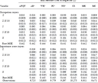
As discussed in IIC, we estimate select log- wage models using subsamples of non-mobile men to determine whether our estimates are infl uenced by job mobility. We select observations for a subsample of “occupation stayers” by allowing each man to contribute wage observations as long as his three- digit occupation remains unchanged relative to his initial observation. We select subsamples of “importance score stayers” by retaining each sample member as long as his raw skill- specifi c importance score does not change by more than 0.1 relative to his initial occupation’s score. Each sub-sample has the same number of men (3,069) as the full sub-sample. The subsub-sample of “occupation stayers” has 8,778 wage observations; sample sizes for “importance score stayers” are tied to the skill measure being used but range from 9,471 for mechanical comprehension to 10,273 for coding speed (see Table 8).
We also estimate select specifi cations for a subsample of men with exactly 12 or 16
years of schooling and for a subsample of observations corresponding to blue- collar or white- collar occupations.13 These subsamples are used for comparison with the fi ndings of Bauer and Haisken- DeNew (2001) and Arcidiacono, Bayer, and Hizmo (2010) although, unlike those authors, we use pooled samples (S = 12 and S = 16; blue- collar and white- collar) and interactions to allow each parameter to vary by type. We also defi ne each “type” to be time- constant for each respondent whereas Bauer and Haisken- DeNew (2001) and Arcidiacono, Bayer, and Hizmo (2010) allow respondents to appear in both subsamples. Our schooling sample consists of 14,979 observations for 1,677 men with 12 years of schooling and 4,516 observations for 560 men with 16 years of schooling; our occupation sample consists of 17,189 observations for 1,900 men in blue- collar occupations and 9,597 observations for 1,264 men in white- collar occupations.
B. Variables
Table 1 briefl y defi nes the variables used to estimate our log- wage models and pres-ents summary statistics for samples described in the preceding subsection. Our depen-dent variable is the natural logarithm of the CPI- defl ated average hourly wage, which we construct from the NLSY79 “rate of pay” variables combined with data on annual weeks worked and usual weekly hours.
For comparability across specifi cations, we always use a uniform set of baseline covariates. We follow convention in using highest grade completed (S) as a measure of productivity that employers observe ex ante.14 Our schooling measure is based on NLSY79 created variables identifying the highest grade completed in May of each calendar year and identifi es the schooling level that prevails at each respondent’s date of school exit. Because we truncate the observation period at the date of school reentry for respondents seen returning to school, our schooling measure is fi xed at its premar-ket level for all respondents, as required by the model; discontinuous schooling is a relatively common phenomenon among NLSY79 respondents (Light 1998, 2001). We also control for a cubic in potential experience (X), which we defi ne as the number of months since school exit divided by 12. In addition, we control for two dummy variables indicating whether the individual is black or Hispanic (with non- black, non- Hispanics serving as the omitted group), interactions between S and these race/ethnic-ity dummies, the interaction between S and X, a dummy variable indicating whether the individual resides in an urban area, and individual calendar year dummies. This baseline specifi cation mimics the one used by AP.
In a departure from prior research on employer learning, we control for
produc-13. Following U.S. Census Bureau definitions, we define a wage observation as white collar if the worker’s initial occupation corresponds to professional, technical, and kindred workers; managers and administrators, except farm; sales workers; or clerical and kindred workers. A wage observation is classified as blue collar if the initial occupation corresponds to craftsmen and kindred workers; operatives, except transport; transport equipment operatives; or laborers, except farm.
tivity correlates that employers potentially learn over time (Z) with eight alternative measures of cognitive skills. Our fi rst measure is the one relied on throughout the existing literature: an approximate Armed Forces Qualifi cations Test (AFQT) score constructed from scores on four of the ten tests that make up the Armed Services Vo-cational Aptitude Battery (ASVAB).15 Our remaining measures are scores from seven individual components of the ASVAB: arithmetic reasoning, word knowledge, para-graph comprehension, numerical operations, coding speed, mathematics knowledge, and mechanical comprehension. We use the fi rst four ASVAB scores because they are used to compute the AFQT score; we include the remaining scores because, along with the fi rst four, they can be mapped with minimal ambiguity to O*NET importance scores.16 We provide the formula for computing AFQT scores and a mapping between ASVAB skills and O*NET measures in Table A1 in Appendix 1.
As detailed in Section II, our use of alternative test scores presents us with a chal-lenge not faced by analysts who rely exclusively on AFQT scores as a proxy for Z: In order to compare estimated coeffi cients for Z·X and Z across test scores and attri-bute those differences to skill- specifi c employer learning and screening, we have to contend with the fact that each Z is correlated with S, X, and other regressors and that these correlations differ across test scores. Table 2 shows correlations between each (raw) test score and S, black, Hispanic, X and IS; because X and IS are time- varying, we use each worker’s initial and fi nal values. Unsurprisingly, each test score is highly correlated with S. These correlations range from a high of 0.645 for mathematics knowledge to a low of 0.426 for mechanical comprehension, which is arguably the most vocationally oriented of our skill measures. Each test score is negatively cor-related with black and Hispanic, and with both initial and fi nal values of X—and for each variable, the degree of correlation again varies considerably across test score.17 Scores for the more academic tests (including mathematics knowledge, arithmetic reasoning, and word knowledge) tend to be highly correlated with skill importance, while scores for vocationally oriented tests (coding speed, mechanical comprehension) are much less—and even negatively—correlated with importance.
To net out these correlations we regress each raw test score, using one observation per person, on each time- invariant regressor (S and the two race/ethnicity dummies) as well as initial and fi nal values for urban status, X, S·X, black·X, Hispanic·X, and the importance score corresponding to the particular test. Because NLSY79 respondents ranged in age from 16–23 when the ASVAB was administered, we also include birth year dummies in these regressions. We then standardize score- specifi c residuals to have a zero mean and standard deviation equal to one for the “one observation per
15. NLSY79 respondents were administered the ASVAB in 1980. All respondents were targeted for this testing—which was conducted outside the usual in- person interviews—and 94 percent completed the test. 16. Our seven skill measures are the only ones satisfying two requirements: (a) they must be measured for NLSY79 respondents prior to the start of the career, and (b) an O*NET measure of skill importance must be available for the skill. Other precareer NLSY79 skill measures (for example, the three remaining ASVAB components and noncognitive skill measures such as locus of control and self- esteem) do not map cleanly into O*NET importance scores. Other O*NET importance scores (for example, physical stamina) are not assessed by the NLSY79.
The Journal of Human Resources
Table 1
Means and Standard Deviations for Select Variables in Alternative Samples
Variable
Full Sample
Occupation
Stayers S = 12 S = 16
Blue Collar
White Collar
Log of CPI- defl ated average hourly wage 1.99 2.01 1.89 2.41 1.92 2.25
(0.54) (0.56) (0.46) (0.53) (0.47) (0.61)
Highest grade completed (S) 12.59 13.09 12.00 16.00 11.80 14.57
(2.17) (2.31) — — (1.49) (2.32)
Years of potential experience (X)a 6.69 4.57 7.08 6.04 6.89 6.25
(4.11) (3.88) (4.13) (3.96) (4.12) (4.05)
S·X / 10 8.35 6.04 — — 8.12 9.02
(5.30) (5.31) (4.97) (5.97)
1 if black 0.25 0.23 0.29 0.16 0.25 0.19
black∙X 1.79 1.07 2.17 1.00 1.78 1.27
(3.71) (2.73) (4.03) (2.83) (3.72) (3.16)
1 if Hispanic 0.16 0.15 0.15 0.08 0.17 0.14
Hispanic∙X 1.11 0.72 1.10 0.50 1.23 0.94
(3.04) (2.32) (3.05) (2.07) (3.21) (2.78)
1 if urban 0.75 0.75 0.73 0.84 0.71 0.83
Raw AFQT score (Z)b 63.83 68.04 60.22 87.22 58.57 78.54
Light and McGee
87
(7.39) (7.60) (6.46) (5.73) (6.57) (7.28)
Word knowledge (WK) 22.88 24.28 21.56 30.82 21.12 27.79
(8.62) (8.32) (8.07) (4.05) (8.33) (7.04)
Paragraph comprehension (PC) 9.45 9.99 8.94 12.87 8.66 11.63
(3.79) (3.74) (3.60) (1.79) (3.64) (3.13)
Numerical operations (NO) 30.35 32.18 29.19 39.31 28.20 36.38
(11.25) (11.20) (10.59) (8.02) (10.70) (10.09)
Coding speed (CS) 38.20 40.79 36.40 50.04 35.27 46.51
(15.63) (15.45) (14.50) (12.55) (14.78) (14.45)
Mathematics knowledge (MK) 12.18 13.41 10.65 19.92 10.39 16.88
(6.30) (6.64) (4.95) (4.86) (5.10) (6.53)
Mechanical comprehension (MC) 14.09 14.86 13.66 17.75 13.44 16.31
(5.59) (5.59) (5.46) (4.49) (5.53) (5.22)
Number of observations 22,907 8,778 11,960 3,313 12,253 6,181
Number of men 3,069 3,069 1,461 480 1,516 953
Notes: All specifi cations also control for Z·X, X2, X3, and calendar year dummies.
a. Elapsed months since fi rst school exit divided by 12.
The Journal of Human Resources
Table 2
Pearson Correlation Coeffi cients for Skill Measures and Select Covariates
Skill Measure S Black Hispanic X0 Xf ISZ
0 IS
Z f
AFQT 0.608 –0.402 –0.108 –0.065 –0.201
Arithmetic reasoning 0.574 –0.374 –0.114 –0.078 –0.191 0.355 0.346
Word knowledge 0.546 –0.395 –0.093 –0.054 –0.195 0.351 0.378
Paragraph comprehension 0.533 –0.334 –0.105 –0.048 –0.173 0.359 0.366
Numerical operations 0.500 –0.297 –0.071 –0.044 –0.144 0.281 0.268
Coding speed 0.470 –0.316 –0.039 –0.057 –0.132 0.099 0.078
Mathematics knowledge 0.645 –0.304 –0.101 –0.080 –0.188 0.293 0.250
Mechanical comprehension 0.426 –0.428 –0.095 –0.058 –0.136 –0.021 –0.057
Notes: The sample consists of one observation for each of the 3,069 men in the full sample. Skill measures are raw (nonstandardized) scores. Potential experience (X) and importance scores (ISZ) correspond to the
person” sample of 3,069 men; the standard deviations continue to be very close to one in the regression sample consisting of 22,907 person- year observations.
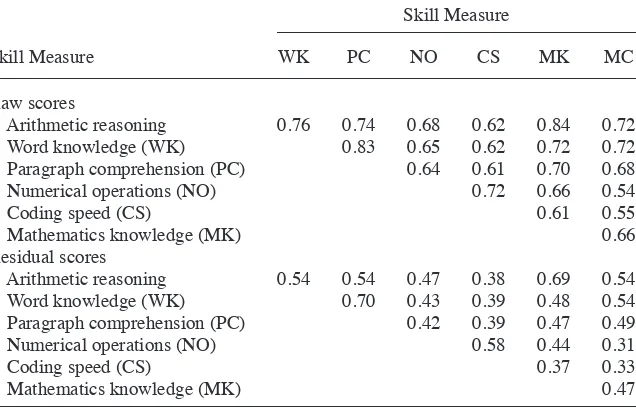
Our use of alternative test scores also compels us to consider whether the seven ASVAB components measure distinct skills or whether they simply provide alternative measures of a single, general skill. In the top panel of Table 3 we demonstrate that correlation coeffi cients among raw scores for the seven tests range from 0.54 to 0.84, with the largest correlations belonging to two pairs: word knowledge and paragraph comprehension, and arithmetic reasoning and mathematics knowledge. The bottom panel of Table 3 shows that most of these correlations fall to 0.30–0.50 when we use residual scores although they remain at about 0.7 for the two pairs just mentioned. Clearly, much of the correlation in the raw scores refl ects the fact that sample mem-bers who are older and/or more highly schooled tend to perform better on all tests. Once those factors are netted out, the dramatically lower correlation coeffi cients in the bottom panel suggest that we are not simply measuring “general skill” with seven different tests—although the skills measured by word knowledge and paragraph com-prehension are undeniably similar, as are those measured by arithmetic reasoning and mathematics knowledge. The evidence in Table 3 suggesting that we are, in fact, mea-suring fi ve distinct skills (“verbal,” “math,” numerical operations, coding speed, and mechanical comprehension) is corroborated by several studies that use factor analysis or item response theory to analyze ASVAB scores (Stoloff 1983; Welsh, Kucinkas, and Curran 1990; Ing and Olsen 2012).
Table 3
Pearson Correlation Coeffi cients for Skill Measures
Skill Measure
Skill Measure WK PC NO CS MK MC
Raw scores
Arithmetic reasoning 0.76 0.74 0.68 0.62 0.84 0.72
Word knowledge (WK) 0.83 0.65 0.62 0.72 0.72
Paragraph comprehension (PC) 0.64 0.61 0.70 0.68
Numerical operations (NO) 0.72 0.66 0.54
Coding speed (CS) 0.61 0.55
Mathematics knowledge (MK) 0.66
Residual scores
Arithmetic reasoning 0.54 0.54 0.47 0.38 0.69 0.54
Word knowledge (WK) 0.70 0.43 0.39 0.48 0.54
Paragraph comprehension (PC) 0.42 0.39 0.47 0.49
Numerical operations (NO) 0.58 0.44 0.31
Coding speed (CS) 0.37 0.33
Mathematics knowledge (MK) 0.47
As a result of correlations among our residual test scores, estimated effects of screening and employer learning for a given skill will potentially refl ect screening and learning with respect to any other skill with a correlated test score. Suppose, for ex-ample, that employers learn about numerical operations over time but not about para-graph comprehension. Given the modest correlation between the test scores for these skills seen in Table 3, our estimates would identify employer learning with respect to paragraph comprehension—but would correctly identify more employer learning for numerical operations than for paragraph comprehension. In general, our estimates will correctly “rank” the degree of learning (and screening) across distinct skills, even if the test score correlations shown in Table 3 cause some estimates to be overstated.18
In another departure from the existing literature, our covariates include occupation- specifi c importance scores (ISZ) for each skill measure except AFQT scores. These
scores, which we construct from O*NET data, represent the importance of each skill measured by the given ASVAB component in the three- digit occupation associated with the current job; we use the fi rst- coded occupation for each job, so ISZ is time-
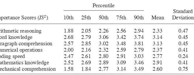
invariant within job. For example, the score for arithmetic reasoning refl ects the im-portance in one’s occupation of being able to choose the right mathematical method to solve a problem while the score for mathematics knowledge measures the importance of knowing arithmetic, algebra, geometry, etc. The importance scores range from one for “not important” to fi ve for “extremely important” and refl ect the average responses of workers surveyed in an occupation.19 Some skills are important in most jobs while others are important in only a few jobs, as the distributions in Table 4 indicate. For instance, paragraph comprehension and word knowledge are “important,” “very
im-18. In principle, we can eliminate correlations among test scores by including all other scores in the regres-sions used to compute skill- specific residual scores. We do not use this strategy due to concerns that “noise” dominates the remaining variation in each residual score. We do not include multiple test scores in a single regression because AP’s test for EL requires scalar measures of Z.
19. See Appendix 1 for additional details on how O*NET creates importance measures and how we construct our IS variables.
Table 4
Importance Score Distributions (Full Sample)
Importance Scores (ISZ)
Percentile
Mean
Standard Deviation 10th 25th 50th 75th 90th
Arithmetic reasoning 1.88 2.05 2.26 2.56 2.94 2.33 0.47
Word knowledge 2.68 2.79 3.06 3.42 3.74 3.14 0.45
Paragraph comprehension 2.57 2.85 3.02 3.48 3.81 3.13 0.45 Numerical operations 2.00 2.16 2.32 2.59 2.79 2.37 0.41
Coding speed 2.47 2.61 2.80 2.91 3.03 2.77 0.24
Mathematics knowledge 2.52 2.69 2.89 3.09 3.46 2.91 0.41 Mechanical comprehension 1.58 1.84 2.77 3.14 3.49 2.60 0.75
portant,” or “extremely important” (scores 3–5) in more than half of all observations in our sample while arithmetic reasoning and numerical operations range from “im-portant” to “extremely im“im-portant” in only about 10 percent of the observations in our sample.
Given that importance scores (ISZ) play such a critical role in our analysis, we
con-clude this section by addressing two questions: Do the scores appear to make sense? What do these scores measure that might be missed by conventional occupation cat-egories? To address these questions, in Table 5 we present importance scores for sev-eral three- digit occupations, along with the mean growth in residual wage variance (GRV) reported in Mansour (2012) for the aggregate occupation group to which the three- digit occupation corresponds. Unsurprisingly, the importance scores for “word knowledge” and “paragraph comprehension” are highest for lawyers and lowest for dancers, truck drivers, and auto mechanics. Similarly, importance scores for “arithme-tic reasoning” and “numerical operations” are highest for mathema“arithme-ticians and lowest for dancers. Coding speed, which is the ability to fi nd patterns quickly and accurately, is more important for key punch operators than for other occupations in our selected group, while mechanical knowledge is most important for auto mechanics. If any sur-prise is revealed by Table 5, it is that basic reading, language, and mathematics skills are deemed to be fairly important in each of these disparate occupations.
Table 5 also illustrates the type of heterogeneity that is captured by ISZ but
poten-tially missed by Mansour’s (2012) occupation- based classifi cation (GRV). A com-parison of secondary school teachers and truck drivers reveals that, unsurprisingly, importance scores for most skills differ dramatically across these occupations. How-ever, these highly dissimilar occupations fall into aggregate occupational groups with identical mean GRV. At the other extreme, physicians and biological scientists fall into aggregate occupations (health diagnosing and natural scientists) with GRV values at opposite ends of the distribution (0.291 versus –0.064), despite the fact that impor-tance scores for these occupations tend to be similar. Auto mechanics and truck drivers make another interesting comparison: Importance scores for most skills are virtually identical for these two occupations and, in this case, they have fairly similar values for GRV. However, mechanical comprehension is extremely important for mechanics and much less so for truck drivers. We use these examples to suggest that a measure of “job type” based strictly on occupation codes (as proxied by GRV) lacks the sub-stantive content embodied in a task- based or skill- based measure (ISZ). Importance
scores suggest that employer learning with respect to word knowledge might be more pronounced for teachers but not for truck drivers because this particular skill is im-portant for teaching. The use of GRV not only predicts identical employer learning for teachers and truck drivers but lacks the “content” to justify why this (or any) similarity might exist.
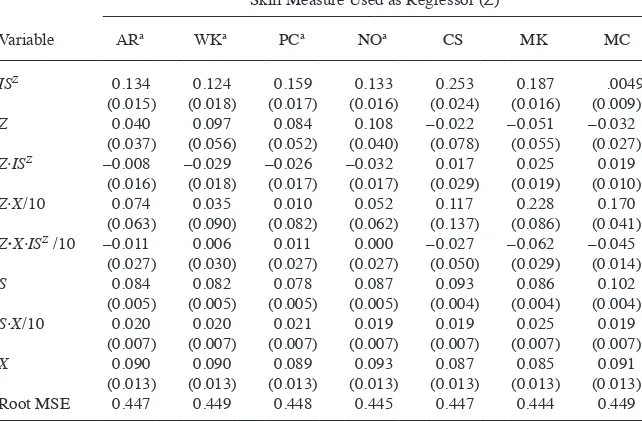
IV. Findings
The Journal of Human Resources
Table 5
Importance Scores and Growth in Variance of Log Wage Residuals (GRV) for Select Occupations
Importance Scorea
Codeb Occupation GRVc AR WK PC NO CS MK MC
031 Lawyer –0.116 2.280 4.525 4.253 2.285 2.780 2.663 1.448
035 Mathematician 0.002 3.875 3.875 3.690 3.565 2.690 4.260 1.490
044 Biological scientist –0.064 3.321 4.193 4.139 3.156 2.988 3.718 1.959
065 Physician 0.291 2.668 4.218 4.184 2.688 3.099 3.023 1.606
144 Teacher (secondary) 0.067 2.876 4.399 4.016 2.655 2.781 3.519 1.796
182 Dancer –0.035 1.630 2.780 3.315 1.755 2.625 2.100 1.200
345 Key punch operator 0.087 2.630 3.710 4.250 2.380 3.750 2.950 1.480
473 Auto mechanic 0.054 2.150 3.127 3.046 2.216 2.820 2.959 3.969
715 Truck driver (light) 0.067 2.005 3.088 2.815 2.253 2.878 2.530 2.765
Notes: High (low) scores for each column are in bold (italics). See Appendix 1 for details on O*NET scores.
a. Importance scores are arithmetic reasoning (AR), word knowledge (WK), paragraph comprehension (PC), numerical operations (NO), coding speed (CS), mathematics knowledge (MK), and mechanical comprehension (MC).
b. 1970 Census three- digit occupation code.
scores for individual components of the ASVAB. In the top panel, we transform each raw test score by regressing it on birth year dummies to account for age differences when the tests were taken, and then standardize the residual scores to have unit vari-ance. In the bottom panel—as well as in all subsequent tables in this section—we switch to the construction method described in IIB1 and IIIB in which residuals are obtained from regressions that also include S, X, ISZ, and other covariates.
We begin by comparing our AFQT- based estimates reported in the top panel of Table 6 to those obtained by AP using a similar specifi cation but data through 1992 only.20
20. As reported in their Table 1, Column 4, AP’s estimates (robust standard errors) for Z, Z ∙ X/10, S and
S ∙ X/10 are 0.022 (0.042), 0.052 (0.034), 0.079 (0.015) and −0.019 (0.012), respectively.
Table 6
Estimates for Log- Wage Model 9 Using Alternative Skill Measures (Full Sample)
Skill Measure Used as Regressor (Z)
Variable AFQT ARa WKa PCa NOa CS MK MC
Z independent of birth year onlyb
Z 0.029 0.033 0.009 0.007 0.042 0.028 0.037 0.022
(0.012) (0.010) (0.009) (0.009) (0.009) (0.009) (0.010) (0.009)
Z·X / 10 0.067 0.059 0.069 0.058 0.059 0.046 0.060 0.055
(0.011) (0.013) (0.013) (0.013) (0.012) (0.012) (0.014) (0.013)
S 0.093 0.093 0.097 0.097 0.092 0.094 0.091 0.095
(0.005) (0.005) (0.005) (0.005) (0.005) (0.005) (0.005) (0.005)
S·X / 10 0.015 0.008 0.007 0.008 0.008 0.011 0.008 0.013
(0.007) (0.007) (0.007) (0.007) (0.007) (0.007) (0.007) (0.007)
X 0.100 0.108 0.107 0.106 0.109 0.104 0.111 0.100
(0.013) (0.013) (0.013) (0.013) (0.013) (0.013) (0.014) (0.013)
Root MSE 0.448 0.450 0.451 0.452 0.448 0.451 0.450 0.451
Z independent of birth year, S, and all other covariatesb
Z 0.023 0.023 0.012 0.007 0.035 0.026 0.026 0.018
(0.007) (0.008) (0.007) (0.008) (0.008) (0.008) (0.008) (0.008)
Z∙X / 10 0.065 0.048 0.053 0.047 0.053 0.042 0.047 0.050
(0.010) (0.011) (0.010) (0.011) (0.010) (0.011) (0.011) (0.011)
S 0.098 0.097 0.098 0.098 0.098 0.098 0.097 0.097
(0.004) (0.004) (0.004) (0.004) (0.004) (0.004) (0.004) (0.004)
S∙X / 10 0.015 0.017 0.017 0.016 0.016 0.017 0.019 0.018
(0.007) (0.007) (0.007) (0.007) (0.007) (0.007) (0.007) (0.007)
X 0.097 0.095 0.095 0.096 0.096 0.095 0.096 0.096
(0.013) (0.013) (0.013) (0.013) (0.013) (0.013) (0.013) (0.013)
Root MSE 0.448 0.450 0.451 0.452 0.448 0.450 0.450 0.451
Notes: The full sample consists of 22,907 observations for 3,069 men. All specifi cations include controls for X2, X3, black, Hispanic, black∙X, hispanic∙X, urban, and year dummies; see Table 7 for additional parameter estimates corresponding to the bottom panel. Standard errors (in parentheses) are robust to clustering on individuals. a. These four ASVAB scores are used to compute AFQT scores.
The Journal of Human Resources
Table 7
Additional Estimates Corresponding to the Bottom Panel of Table 6 (Full Sample)
Skill Measure Used as Regressor (Z)
Variable AFQT AR WK PC NO CS MK MC
Constant 0.249 0.242 0.240 0.230 0.238 0.241 0.234 0.239
(0.081) (0.081) (0.081) (0.081) (0.080) (0.080) (0.081) (0.081)
X2 / 10 –0.072 –0.071 –0.071 –0.070 –0.071 –0.071 –0.071 –0.070
(0.013) (0.013) (0.013) (0.013) (0.013) (0.013) (0.013) (0.013)
X3 / 100 0.017 0.016 0.016 0.016 0.016 0.016 0.017 0.016
(0.006) (0.006) (0.006) (0.006) (0.006) (0.006) (0.006) (0.006)
Black –0.080 –0.079 –0.081 –0.079 –0.080 –0.079 –0.078 –0.080
(0.017) (0.017) (0.017) (0.017) (0.017) (0.017) (0.017) (0.017)
Black·X / 10 –0.013 –0.014 –0.013 –0.014 –0.014 –0.014 –0.014 –0.014
(0.002) (0.002) (0.002) (0.002) (0.002) (0.002) (0.002) (0.002)
Hispanic –0.015 –0.014 –0.014 –0.013 –0.013 –0.012 –0.015 –0.012
(0.024) (0.024) (0.024) (0.024) (0.024) (0.024) (0.024) (0.024)
Hispanic·X / 10 0.000 –0.000 0.000 –0.000 –0.000 –0.000 0.000 –0.000
(0.003) (0.003) (0.003) (0.003) (0.003) (0.003) (0.003) (0.003)
Urban 0.089 0.092 0.089 0.090 0.092 0.092 0.090 0.091
(0.013) (0.013) (0.013) (0.013) (0.013) (0.013) (0.013) (0.013)
Our estimated coeffi cient for Z ∙ X/10 (0.067) is larger than the estimate reported by AP (0.052) while our estimated coeffi cient for S ∙ X/10 (0.015) is precisely estimated and of the opposite sign compared to AP’s (imprecise) estimate of –0.019. Because our AFQT- based estimated coeffi cients for Z ∙ X are positive, we join AP in fi nding support for employer learning—but not in fi nding support for statistical discrimination.
When we replace AFQT scores with individual ASVAB scores in the top panel of Table 6, the estimated coeffi cients for Z ∙ X range from 0.046 for coding speed to 0.069 for word knowledge. It is diffi cult to interpret these differences because, as discussed in IIB, each estimated coeffi cient refl ects covariances between Z and other regres-sors, including S; as indicated by Table 2, these covariances differ substantially across test scores. If we were to ignore these confounding covariances we would conclude that employer learning is most pronounced for word knowledge and least pronounced for coding speed and mechanical comprehension, which are the only two tests under consideration that measure vocational skill rather than general verbal and quantita-tive skills.21 This “straw man” result is surprising insofar as we might expect word knowledge to be a skill that workers can accurately signal to employers ex ante while vocational skills would be among the skills employers learn over time by observing performance.
However, such judgments should be based on the bottom panel of Table 6, where we use the portion of Z that is orthogonal to S, X, ISZ, and other regressors. We can
now apply the expression for B3t in Equation 11, which tells us that a positive
esti-mated coeffi cient for Z ∙ X is consistent with employer learning and that the magnitude of each estimate is a direct measure of employer learning. While each estimated Z ∙ X coeffi cient continues to be positive in the bottom panel, we cannot reject the null hy-pothesis that all eight estimates are identical (nor can we reject the null hyhy-pothesis that any pairwise difference is zero). Stated differently, we fi nd evidence of employer learning for all eight skill measures but no evidence that the degree of employer learn-ing is skill- specifi c. The (statistically signifi cant) difference in the top panel between the smallest estimated Z ∙ X coeffi cient and the largest is entirely attributable to the fact that coding speed has a relatively small correlation with S while word knowledge has a large correlation with S (Table 2).22
The estimates in the bottom panel of Table 6 are noteworthy for two additional reasons. First, the estimated coeffi cients for Z range from a statistically insignifi cant 0.007–0.012 for paragraph comprehension and word knowledge to a precisely esti-mated 0.035 for numerical operations. As shown by expression B30 in Equation 12,
these estimates refl ect the extent to which premarket information other than schooling is correlated with Z (Szq) and the importance of Z in determining productivity ( z).
We can conclude, therefore, that word knowledge and paragraph comprehension are less screenable and/or less important than other skills. Second, the estimated coeffi -cients for S ∙ X are small in magnitude but uniformly positive and statistically signifi
-21. While we fail to reject the joint hypothesis of equality of the estimated Z ∙ X coefficients in the top panel of Table 6, the pairwise difference between the estimated word knowledge and coding speed Z ∙ X coefficients is statistically significant.
22. When we construct standardized, residual test scores from regressions of Z on birth year dummies and S
cant. This again contradicts the model’s prediction ( per the expression for B
1t in
Equation 11) that the relationship between S and log- wages should not change with experience. As noted in IIC (following Farber and Gibbons 1996), a positive S- X slope is consistent with a feature of wage determination abstracted from in the model—namely, that highly schooled workers invest more intensively than their less- schooled counterparts in on- the- job training and/or receive a higher return to these skill investments.23
Before proceeding to a discussion of how skill importance affects our inferences, we discuss the robustness of the estimates reported in the bottom panel of Table 6. In results available from the authors, we experimented with nonlinear skill- experience gradients (Z ∙ X2) for the model specifi cations shown in Table 6 given that Lange (2007) and Arcidiacono, Bayer, and Hizmo (2010) fi nd that most employer learning occurs in the fi rst few years of the labor market career. In no instance did this added fl exibility affect our inferences.
Table 8 shows estimates for log-wage Model 9 based on subsamples of “occupation stayers” and “importance score stayers” described in IIIA. Given that job mobility— especially toward jobs that place greater importance on the skill measured by test score Z—can produce a positive estimated Z- X slope in the absence of employer learning, our goal is to assess the potential infl uence of mobility on our “full sample” estimates (Table 6) by comparing them to estimates based on subsamples of workers who do not change occupations, or who do not change occupations “enough” for the Z- specifi c im-portance score to change. Both sets of estimates in Table 8 reveal that job mobility has little effect on the full sample estimates. In particular, we fail to reject the null hypoth-esis that all seven estimated Z·X coeffi cients are equal in both the “occupation stayer” and “importance score stayer” samples. In a few instances the estimated coeffi cient for Z·X changes noticeably relative to the Table 6 estimates. For example, in the “impor-tance score stayer” sample the estimated arithmetic reasoning parameter increases from 0.048 (Table 6) to 0.065 (Table 8) while the estimated math knowledge parameter falls from 0.047 to 0.030; only for these two skills do we fail to reject the pairwise equality of the estimated coeffi cients for Z·X. Overall, the fi nding that employer learning does not differ signifi cantly across test scores continues to hold in samples of nonmobile workers, indicating that job mobility does not signifi cantly affect our fi ndings.
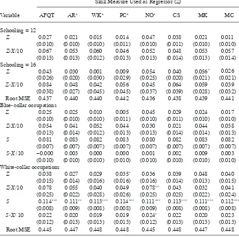
In Table 9, we present estimates for log-wage Model 9 based on a subsample of men with S = 12 or S = 16 and a subsample of observations associated with blue- collar or white- collar occupations; for each subsample, we allow every parameter in the model to differ by “type.” These estimates permit comparison with the fi ndings of Arcidiacono, Bayer, and Hizmo (2010), which identifi es S- specifi c parameters using the NLSY79, and Bauer and Haisken- DeNew (2001), which identifi es parameters for blue- collar and white- collar workers using German Socioeconomic Panel Study data.
The top panel of Table 9 reveals that the estimated Z·X coeffi cients are statisti-cally indistinguishable for men with 12 years of schooling and men with 16 years of schooling for each test score. This fi nding contrasts starkly to evidence in Arcidiacono,