Full Terms & Conditions of access and use can be found at
http://www.tandfonline.com/action/journalInformation?journalCode=ubes20
Download by: [Universitas Maritim Raja Ali Haji] Date: 12 January 2016, At: 23:52
Journal of Business & Economic Statistics
ISSN: 0735-0015 (Print) 1537-2707 (Online) Journal homepage: http://www.tandfonline.com/loi/ubes20
Monetary Policy in a Markov-Switching Vector
Error-Correction Model
Neville Francis & Michael T Owyang
To cite this article: Neville Francis & Michael T Owyang (2005) Monetary Policy in a Markov-Switching Vector Error-Correction Model, Journal of Business & Economic Statistics, 23:3, 305-313, DOI: 10.1198/073500104000000325
To link to this article: http://dx.doi.org/10.1198/073500104000000325
Published online: 01 Jan 2012.
Submit your article to this journal
Article views: 133
View related articles
Monetary Policy in a Markov-Switching Vector
Error-Correction Model: Implications for the
Cost of Disinflation and the Price Puzzle
Neville F
RANCISDepartment of Economics, Lehigh University, Bethlehem, PA 18015
Michael T. O
WYANGResearch Department, Federal Reserve Bank of St. Louis, St. Louis, MO 63102 (owyang@stls.frb.org) Monetary policy vector autoregressions (VARs) typically presume stability of the long-run outcomes.
We introduce the possibility of switches in the long-run equilibrium in a cointegrated VAR by allowing both the covariance matrix and weighting matrix in the error-correction term to switch. We find that monetary policy alternates between sustaining long-run growth and disinflationary regimes. Allowing state changes can also help explain the price puzzle and justify the use of commodity prices as a corrective measure. Finally, we show that regime-switching has implications for disinflationary monetary policy and can explain the variety of sacrifice ratio estimates that exist in the literature.
KEY WORDS: Cointegration; Markov switching; Monetary policy; Price puzzle; Sacrifice ratio.
1. INTRODUCTION
Changes in monetary policy can occur in either the im-plementation of policy (shocks) or the objectives of policy (regimes). The former are typically modeled as vector in-novations to a vector autoregression (VAR) in which mon-etary policy is identified by structural restrictions on the contemporaneous impacts of the variables (e.g., Sims 1992) or restrictions on the long-run effects of shocks (e.g., Blanchard and Quah 1989). This so-called “structural VAR” literature has identified a number of stylized facts resulting from the imple-mentation of monetary policy and has spawned a vast literature (see Bernanke and Mihov 1998; Christiano, Eichenbaum, and Evans 1999 for surveys).
More recently, switching monetary policy regimes have gar-nered some attention (Clarida, Galí, and Gertler 2000; Dennis 2001; Hanson 2002a; Boivin and Gianonni 2002). Policy regimes involve switches in the policy rule that reflect, for example, changes in the policy maker’s reaction to deviations from the target inflation rate or output growth rate. These stud-ies are aimed at finding persistent changes in policy that re-sult, for example, from changes in central bank leadership or transparency. These regime changes can have a large effect on the volatility of money, interest rates, and output. For exam-ple, Clarida et al. (2000) showed that a switch in the objectives of monetary policy post-1982 has resulted in a more stable, inflation-controlling policy. Dennis (2001) argued that a change in policy maker preferences has shifted the post-1979 inflation target down from over 7% to under 2%. Hanson (2002a) ex-amined whether a change in Fed policy was the cause of in-creased instability in the late 1970s and early 1980s. Boivin and Giannoni (2002) considered whether the Fed’s effective-ness has changed in the postwar period.
A new branch of literature has begun to simultaneously examine both regime changes and policy shocks (see, e.g., Bernanke and Mihov 1998; Owyang 2002; Sims and Zha 2002). These authors show, among other things, that the stance of monetary policy is important not only to the policy maker’s
response to the exogenous economic shocks (e.g., the Taylor rule), but also to the contemporaneous effects of the monetary policy innovations (i.e., the monetary shock itself ). What they do not address are the long-run objectives and impacts of mon-etary policy. We investigate those long-run impacts here. Our long-run identification is achieved through the long-run impact matrix of a vector error-correction model (VECM). Short-run identification is achieved by making standard assumptions of how monetary policy impacts other economic variables of in-terest and by similar assumptions about the information set of the Fed.
Our approach incorporates regime switches in the long-run relationships through the weighting matrix of the error-correction term. Gregory and Hansen (1996) also looked at regime switches in the cointegrating vector but made no dis-tinction between the weighting matrix and the long-run equilib-rium (see also Hall, Psaradakis, and Sola 1997; Clarida, Sarno, Taylor, and Valente 2003; Paap and van Dijk 2003 for recent work using Markov switching in an error-correction frame-work). We find it natural to assume that the long-run relation-ships between the cointegrated variables remain the same across states but that the weighting term is state-dependent. Modeling the weighting matrix as state-dependent allows variables to re-spond differently to monetary policy shocks, even in the long run. This lends itself to plausible economic interpretation and at the same time preserves the Engle and Granger (1987) no-tion of cointegrano-tion.
The article proceeds as follows. Section 2 provides a brief motivation for our approach. Section 3 presents a VECM for monetary policy, with Markov switching in the weighting ma-trix for long-run impacts and regime-dependent heteroscedas-ticity, and outlines the estimation technique. Section 4 discusses
© 2005 American Statistical Association Journal of Business & Economic Statistics July 2005, Vol. 23, No. 3 DOI 10.1198/073500104000000325
305
306 Journal of Business & Economic Statistics, July 2005
the results of the estimation. Section 5 considers the implica-tions of the switching model in the context of the price puz-zle. Section 6 examines the sacrifice ratio and the consequences for disinflationary policy brought about by the presence of the switching process governing the weighting matrix. Section 7 concludes.
2. MOTIVATION
To motivate our approach, we briefly present our empirical model here; we give a more detailed version later. Our model is the following VECM, which allows for different states of the economy:
whereStdenotes the period-tstate. In principle, we could allow
part or all of the coefficient matrix to switch independently or with the error-correction term. However, we are interested in changes in the adjustment to the long-run equilibrium and thus restrict our attention to switching in the error-correction term.
This modeling approach partially overcomes the rational ex-pectations critique of models of this nature. The basic rational expectations argument is that in producing impulse responses, VAR (and structural VAR) models look at responses to shocks that are outside the realm of such models. That is, these mod-els look at responses to shocks assumed not to have happened at the time of modeling. To compound matters, these models further assume that the nonpolicy component of the economy is naive about any change in policy that may have taken place; this is so because the coefficient matrix in the VAR is invariant to any switches in policy regime. Our approach does not suffer the same fate. We not only allow the nature of the shock to vary across states through the state-dependency of the error term, but also allow individuals’ responses to the structural shocks identi-fied to be state-dependent by allowing for a different coefficient matrix in each of the states. In this way, individuals “correctly” respond to monetary or any other shocks. Sims (1986) com-pared the rational expectations approach and the VAR method-ology when it comes to forecasting and policy analysis.
Our approach allows for a variety of interpretations regarding the response to monetary policy and is not limited to changes resulting only from switches in the policy maker’s decision rule. Whereas we will often, for the purposes of exposition, attribute changes in the “nonpolicy” response to switches in the speed of adjustment of inflation expectations, we allow for alterna-tive interpretations. Specifically, changes in adjustment speed can result from sectoral shifts (Ramey and Shapiro 1998) or changes in policy maker credibility (Faust and Svensson 1998).
3. MODEL AND ESTIMATION
This section presents a more detailed version of our model-ing approach along with our identification scheme. We adopt some of the more common assumptions used in the identifica-tion of the impact matrix of VAR monetary models. The re-sult is a benchmark recursive model. Thus long-run dynamics obtain (solely) through the error-correction term, St, which
includes both the regime-switching weighting matrix,αSt, and the regime-invariant cointegrating vector,β. We combine both the short-run dynamics, adopted from standard models in the monetary policy literature, and the aforementioned long-run dynamics in a Markov-switching framework. This allows us to examine the state-dependent responses to monetary policy shocks.
3.1 Model
Consider the following Markov-switching VECM (MSVECM):
vector of differenced variables of interest,cis a vector of inter-cepts, theŴi’s arem×mparameter matrices, andStare state-dependent covariance matrices. St are the state-dependent long-run impact matrices defined by ther×mmatrix of coin-tegrating vectors,β, and them×rstate-dependent weighting matrix,αSt. Thus we have
St=αStβ
′.
We assume thatStis a two-state first-order Markov process in
whichSt∈ {0,1}is governed by the transition kernelP, whose
where any switch in the cointegrating relationship is restricted to the weighting matrix,αSt.
The framework (1) can be readily expanded to incorpo-rate switches in the intercept term or the coefficient matrices. We forgo analysis of switching in these components to focus on long-run dynamics. (We considered simultaneous switching in the weighting matrix and the intercept term. We found that including switching in the intercept term reduces the estimated number of periods in the transitory state and prevents reason-able estimates of the model dynamics.)
Switching inSt can be interpreted as switching in the coin-tegrating vectors, the weighting matrix, or both. We note that these approaches are de facto equivalent. However, our interpre-tation of switches in the error-correction term implies a single set of long-run relationships and preserves the Engle–Granger notion of cointegration. In our framework, switches can be in-terpreted as differences in the rate at which the long-run rela-tionships obtain.
We propose that allowing switches only in the weighting ma-trix is not overly restrictive and provides some further inter-pretation for our approach. The first reason for confining the nature of the switches is computational convenience. We find that the model becomes intractable if we allow all of the coef-ficients in the MSVECM to be state-dependent. Allowing for switching in more parameters also confines us to models hav-ing fewer variables. We argue that such a sacrifice is not too great, because additional variables provide us with more dy-namics that would otherwise be absent from a model allowing
for more switches but fewer variables. Second, if we were to map back to the reduced form of the model, then it would be-come apparent that differences between states arise through the coefficient on the first lag of the data matrix (this is how the weighting matrix, αSt, can be state-dependent, whereasŴi is
not). For lower-order systems, this should prove not too restric-tive, becauseA1, the lag-one coefficient from the reduced form of the model, would figure prominently in the error-correction term. The error-correction term isI−ki=1Ai from the
struc-tural model.
We offer as further motivation some other potential interpre-tations of the form of the model. Our preferred interpretation is that the long-run relationship between the variables,β′yt−1,
is invariant to the state of the economy; however, the weights given to each relationship,αSt, are state-dependent. This
im-plies that shocks to the system could potentially have different long-run effects across states, throughαSt, while maintaining
any long-run relationship among the variables. For example, a shock to monetary policy will have different long-run ef-fects on, say, output growth, depending on whether the Fed targeted inflation or output. There are two things at work here: the long-run response to shocks and the cointegrated relation-ship. We can have the cointegrated relationship, β′yt−1,
un-changed while having different long-run responses to shocks. This is due to the fact that the long-run response coefficient is St =αStβ
′,which is a function of the switching elements (see
Hamilton 1994, pp. 579–581, for the long-run response matrix). The nature of the impulse responses thus depends on the Fed’s preference at the time of the shock. A second interpre-tation is thatαStcould reflect the rate at which people learn the
nature of the shock to the Fed’s policy rule. The slower the rate of learning, the greater the impact of shocks to the Fed’s pol-icy rule, implying more persistence in the impulse responses. The weighting coefficient could also be interpreted as indicat-ing the amount of relative frictions that exist in each state. In states where there are more frictions, the responses to monetary shocks will be curtailed.
Finally, we cannot rule out the possibility thatαStcould
cap-ture the nacap-ture of nonpolicy instruments across states. That is, we should expect different responses to monetary policy if the mixture of nonpolicy instruments changes. This latter interptation is outside the scope of this article, because it would re-quire us to redefine the number of states. That is, the states would be a mixture of both policy and nonpolicy instruments resulting in spolicy∗snonpolicy states, instead of spolicy states. We ignore this latter interpretation for now and treat all non-policy instruments as if they were one.
3.2 Estimation
The data are the monthly coincident indicators index, the per-sonal consumption expenditure (PCE) chain price index, and the federal funds rate from 1960:01 to 2003:08. Each of the first two variables are entered in log levels. The model (2) can be estimated using an iterative three-step Gibbs sampling pro-cedure (e.g., Krolzig 1996, 1997). First, we determine the num-ber of cointegrating relationships using Johansen’s maximum eigenvalue procedure. This two-step procedure is adopted from the work of Saikkonen (1992) and Saikkonen and Luukkonen
(1997) to obtain estimates of the cointegrating vectors,β. These authors showed that the Johansen procedure estimates consis-tent cointegrating vectors even in the presence of switching. Then, conditional on these cointegrating vectors, define the
(km+1+2r)×1 vector
Xt=[ 1 yt−1 · · · yt−k β′yt−1(1−St) β′yt−1St]′.
Then the system (2) can be stacked,
Y=X+ε, (3)
Given (3), a matrix of cointegrating vectors β, and a series of statesST = {S1,S2, . . . ,ST}, we draw the parameter values
from the posterior normal-inverted Wishart distribution with priorsν01,ν02,N0,Z0,W01,andW02. The priors that we use are uninformative. Alternative priors that could take advantage of the Bayesian methodology might use, for example, the Sims– Zha (Sims and Zha 1998) prior. In that case, the prior accounts for possible (unestimated) cointegrating vectors. Because we use uninformative priors, we model the cointegrating vectors explicitly.
At each iteration,,1,and2can be drawn from a distrib-ution with degrees of freedomν, precision matrixN, parameter meansZ, and covariance matricesW1andW2, defined by
ν1=ν01+T1,
308 Journal of Business & Economic Statistics, July 2005
andp(St−1|yt−1,,1,2)is taken from each previous itera-tion (see Hamilton 1989; Kim and Nelson 1999).
The transition probabilities,pij=Pr[St=i|St−1=j], are also derived from the estimation algorithm. Although we forgo for-mal discussion of their estimation, we note that they are drawn from posteriors formed from beta-conjugate distributions.
To satisfy the Lucas critique, we require that the state process depend on the underlying stochastic process, ε (see, e.g., Hamilton 1995). We partially accomplish this in two ways. First, the posterior distribution for the state process (5) is a func-tion of the state-dependent variance–covariance matrix. Sec-ond, the data used in the filtering of the state process are the same data used in the estimation of the state-dependent coeffi-cient matrices in the VECM.
3.3 Identification
Identification of the model implies two steps: identification of the long-run relationships through the set of cointegrating vectors and identification of the short-run effects through the contemporaneous impact matrix. We discussed the former ear-lier. In a three-variable model, our short-run identification con-sists of a Cholesky ordering of the system with the variables ordered: output, prices, and federal funds rate. This implies that the monetary authority takes both output and prices into con-sideration when setting policy, but that policy does not impact output and prices contemporaneously.
We use the recursive form of identification to evaluate the reasonableness of the results using our methodology with the most basic form of identification. More complicated forms of identification came about because simpler identifying assump-tions could not deliver impulse responses that were consistent, or considered consistent, with monetary policy. Our aim is to see how much mileage we get from our methodology with as few structural assumptions as possible.
4. EMPIRICAL RESULTS
In this section we examine monetary shocks in a three-variable cointegrated extension of common VAR models, which account for, among other factors, the changes in inflation ex-pectations. We impose a two-state restriction on the underly-ing Markov process for tractability. Although we recognize that this is limiting, we believe that it is illustrative of how a model of this nature can partially characterize a solution to the ra-tional expectations critique. As a test, we estimated a three-state model. Under our specification, the filter did not identify enough periods in the third state to estimate that state’s para-meters with any confidence. We therefore leave higher-order Markov models for future research.
4.1 States
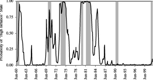
The state process is shown in Figure 1, in which the proba-bility that the economy is in state 2 is indicated on they-axis. This regime could be interpreted as a high inflation target or high inflation expectations regime. This figure corresponds to the posterior probabilities governing the weighting matrix in the error-correction term and shows that this cointegration relation-ship undergoes five significant periods of change. The timing of
Figure 1. State 2 Posterior Probabilities: Smoothed Probabilities, Pr[St=2|Y1, . . . , Yt] (solid line); NBER Recession (shaded regions).
switches to the high inflation expectations state tends to be cor-related with events such as oil shocks and recessions, although not exclusively so. For example, the 1973–1975 recession and the Volcker disinflation are clearly identified by the underlying state process.
Most of the turning points are related to events coincident with large increases in prices. These include the consumer price index reaching a new peak in 1960, the devaluation of the dollar and a spike in inflation in early 1969, and a farm recession and oil price shock in the mid-1980s. These posterior state proba-bilities are consistent with the findings of other monetary policy models (Owyang 2002; Sims and Zha 2002) and recession-dating models (Hamilton 1989).
Table 1 shows two long-run relationships, with cointegrating vectorsβ1andβ2, that are fixed across regimes; it also provides the weighting matrices for these relationships that vary across regimes. The absolute size of the weights is greater in state 1 than in state 2, implying that the rate of convergence (or rate of learning) differs across states. Moreover, the nature of the long-run response—or, to be more precise, the transition to the long-run equilibrium—associated with the first cointegrating relationship differs across states. Finally, Table 1 provides es-timates of the transition probabilities for each state. We note in particular that each state, characterized by transition probabili-ties below .1, is relatively persistent.
Table 1. Estimation Results
Y P R
Cointegrating β1b −2.137 .1099 .1904 vectorsa β2c .3584 −.1958 .2755 Weighting α1(St=1) .0067 .1044 −.2729
matricesd (.037) (.062) (.217)
α1(St=2) −.022 −.0971 .4275
aUnnormalized cointegrating vectors from Johansen’s max eigenvalue procedure. bNull of no cointegrating vector rejected at 5%.
cNull of only one cointegrating vector rejected at 5%. d60% coverage intervals in parentheses.
4.2 Transition Dynamics
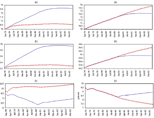
To evaluate the effect of a change in state, we conduct the counterfactual state-switching experiments to demonstrate the model’s transition dynamics. These switches might be viewed as either the economy’s assimilation of a change in the Taylor rule (e.g., Clarida et al. 2000) or the inflation objective (e.g., Dennis 2001). We initialize the model with 1978 data and set the state to 1. We then switch to state 2 and observe the tran-sition dynamics in the absence of shocks. After 24 periods, we switch the regime back to state 1. This exercise (experiment A) is shown as the solid line in Figure 2. This contrasts with the model remaining in state 1 for all time (experiment B), the dot-ted line in Figure 2. Although the recession in A is deeper, the policy maker is able to lower prices without exogenous mone-tary shocks. Moreover, in A, the Fed’s policy appears more anti-inflationary at the outset and, thus produces a steeper recession and more rapid disinflation. Because this outcome is produced in the absence of monetary shocks, only a limited number of interpretations can explain the results. Changes in Fed prefer-ences or changes in the inflation target can explain the switch in the expected path of the funds rate.
(a)
(b)
(c)
Figure 2. State Transition Experiments 1 for (a) Output, (b) Price, and (c) Federal Funds Rate: Experiment A (switches from state 2 to state 1 in January 1981, solid line); Experiment B (remains in state 1 for all time, dotted line).
A second set of experiments demonstrates the effect of re-maining in state 2 for all time. Figure 3 shows the results of these experiments; the solid line indicates the case in which the long-run relationship switches to state 1 after 24 periods (ex-periment C), and the dotted line represents the path governed by state 2 for all time (experiment D). This set of experiments further verifies the nature of the long-run relationships in this model. State 2 represents an upward trend in both prices and output, as well as a sustained expansionary monetary policy ex-hibited by an ever-decreasing funds rate. We can interpret the inflation regime (state 2) as one in which the Fed has either established a new, higher inflation target or is sacrificing price stability to increase growth. Further, we can interpret the growth regime (state 1) as the Fed adopting either sustained inflation-neutral or actively contractionary monetary policy under low inflation expectations.
Although in the preceding experiments it may appear that the regimes are simply manifestations of contractionary and expan-sionary policyshocks, we reiterate that the state changes reflect changes in thestanceof policy. The idea of asustainedpolicy stance is important to our interpretation. These regimes are sup-ported not by contractionary or expansionary shocks, but rather
(a)
(b)
(c)
Figure 3. State Transition Experiments 2 for (a) Output, (b) Price, and (c) Federal Funds Rate: Experiment C (switches from state 2 to state 1 in January 1981, solid line); Experiment D (remains in state 2 for all time, dotted line).
310 Journal of Business & Economic Statistics, July 2005
by a revision of preferences or expectations. We explore the ef-fect of monetary policy shocks in the next section.
4.3 Responses to Policy Shocks
Consider the short-run response to a 1–standard deviation shock to the federal funds rate. These impulse responses are generated conditional on the state; that is, we assume that if the shock is generated in state 1, then it is transmitted through state 1. Although we acknowledge that this is a restriction, the state-dependent impulse responses and the state transition ex-periments are sufficient to describe the majority of the model’s short-run dynamics.
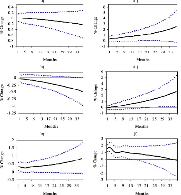
Figure 4 shows the effect of a contractionary monetary policy shock (a 100–basis point increase in the federal funds rate). In state 1, the contractionary shock has the anticipated effect on output—the increase in the funds rate induces a recession. The effect on output is relatively weak. The recession is deflationary, causing a reduction in prices over the 4-year period.
The contractionary monetary shock in state 2 keeps the funds rate strictly positive for 1 year. In contrast to state 1, the cen-tral tendency is to fully reverse the shock after approximately
30 months. Also in state 2, output is bolstered by the policy reversal and rises (weakly) over 48 months. This causes prices to continue to rise; the policy shock stems inflation for the first few years, but the reversal allows prices to continue to increase.
5. THE PRICE PUZZLE
Originally identified by Sims (1992), VAR studies of mone-tary policy have shown that a contractionary shock to the fed-eral funds rate results in a temporary (often lasting a year or more) increase in the aggregate price level. This “price puzzle” has remained a question mark in the identification of monetary policy shocks, because most researchers believe that identifi-cations that exhibit the phenomenon are incorrect. Sims recog-nized that including a commodity price index (PCOM) in the estimation eliminates the increase in prices associated with a contractionary monetary shock. Hanson (2002b), however, ar-gued that adding a PCOM to solve the price puzzle is ad hoc and theoretically unappealing.
Proponents of including PCOM might argue that PCOMs capture inflation expectations. Our approach is to model in-flationary expectations (or at least take them into account) by
(a) (b)
(c) (d)
(e) (f)
Figure 4. Impulse Responses: (a) Output (state 1), (b) Output (state 2), (c) Price (state 1), (d) Price (state 2), (e) Federal Funds Rate (state 1), (f) Federal Funds Rate (state 2): 60% Coverage Intervals Are Shown.
allowing both shocks (authority side) and responses (agents side) to change accordingly. Modeling the VAR in this way al-lows inflationary expectations to vary across states. Thus we do not need a PCOM to reflect expectations. Because we model both the monetary authority’s and respondents’ expectations, we have a more theoretically interpretable explanation. In re-cent work, Owyang and Ramey (2004) discovered that switches from an inflation-hawk policy regime to an inflation-dove pol-icy regime can lead to the hump-shaped price response that characterizes the price puzzle. We conjecture that the price puz-zle may in fact stem from the standard VAR’s inability to effec-tively model these types of switches.
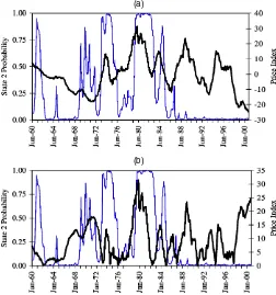
We also contend that commodity prices model inflation ex-pectations corresponding to Fed policy. To illustrate this point, we plot the detrended industrial commodity price index against the state-switching process; results were similar when using the Dow Jones commodity price index for a smaller sample. Figure 5(a) shows that the majority of the state switches coin-cide with (or predate) major commodity price changes in either direction. For example, the switch in the early 1970s coincides with a fall in commodity prices, whereas the switch in the early 1980s coincides with a rise in prices. The correlation between the state-switching process and the detrended PCOM is .34. We consider this significant, given that we restricted our model to only two states of nature and also recognize that not every (major) price change necessarily implies a new state. That is, price changes could also be due to, say, demand factors and are not necessarily limited to policy actions. Figure 5(b) plots the
(a)
(b)
Figure 5. Graphs Plotting the Posterior Probability of State 2 Against (a) (linear) Detrended Commodity Prices (bold line), With Correlation=.34, and (b) the Absolute Movements in Commodities Prices Around Its Trend (bold line), With Correlation=.14. Commodi-ties prices are taken from the Journal of Commerce’s industrial price index.
absolute value of the detrended price series against the state-switching process to highlight the fact that switches in states invariably coincide with major price movements.
The conclusion that we draw from this simple exercise is that including a PCOM in structural VARs is appropriate because they proxy for policy-related changes in inflationary expecta-tions. However, including a PCOM does not lead to an obvious economic interpretation. The problem remains that responses to monetary policy vary depending on the goals of the Fed and how quickly such goals are realized by respondents. That is, tra-ditional VARs provide us with only one response for, say, infla-tion, even though there are as many responses as there are states (as in the MSVECM framework). It comes as no surprise to us that PCOMs play such a role, because, in our opinion, they are the most responsive, and thus the most likely, candidates to re-flect the state process. Therefore, considering monetary policy in a state-switching framework resolves the price puzzle with-out the inclusion of a PCOM and at the same time provides impulse responses that are more accurate representations of the nature of policy and the goals of the Fed.
6. THE COST OF DISINFLATION
A number of studies have used structural models to assess the output or employment loss caused by disinflationary mone-tary policy (see, e.g., Okun 1978; Fuhrer 1994, 1995; Cecchetti and Rich 2001). These studies have constructed “sacrifice ra-tios” that measure the cumulative increase in unemployment or loss of output associated with each percentage point of policy-induced inflation reduction. In particular, there is a rough con-sensus that a 1% reduction in inflation increases cumulative unemployment by about 2 percentage points per year. Cecchetti and Rich (2001) found sacrifice ratios in terms of output loss over a 2-year horizon ranging from .62 to 3.71 using three struc-tural VARs of monetary policy. Recently, Filardo (1998) con-cluded that the sacrifice ratio varied across different regimes, and interpreted these regimes as growth states in which mone-tary policy produced different effects.
To calculate the sacrifice ratio, we can assess the output cost of a temporary disinflationary monetary shock within a single regime. Our model has the additional advantage of allowing us to measure the cost of disinflation occurring as a result of switches between regimes. This also allows us to reconcile a number of different, seemingly contrary, facts derived from the literature. First, our model supports multiple “within-regime” sacrifice ratios, which may explain the different numbers that others have estimated using structural models with alternative assumptions. This is also consistent with Fuhrer’s (1994, 1995) and Filardo’s (1998) claims of multiple structural breaks in sac-rifice ratio estimation. Further, our model reconciles, in an intu-itive manner, a low estimated sacrifice ratio without forfeiting the high-output-loss recessions that were seemingly driven by the Volcker disinflation (see Owyang and Ramey 2004).
We posit two distinct disinflationary episodes, one driven by a policy shock and one driven by a change in regime. If the state truly is a reflection of the underlying inflation expecta-tions, then the difference in the two disinflationary forces is apparent. Within a regime, the policy maker disinflates under
312 Journal of Business & Economic Statistics, July 2005
Table 2. Costs of Disinflation
Sacrifice ratio∗
Within state 1 2.16
Within state 2 3.6
From state 1 to state 2 1.33
From state 2 to state 1 1.19
∗Percent growth lost per percentage point inflation reduction per year at 5-year horizon.
fixed inflation expectations. Fixed expectations build in infla-tion persistence, and as a result, the disinflainfla-tion is costly. Across regimes, the policy maker has the benefit of shifting expecta-tions, which can in and of themselves aid disinflation. Lower expectations can support a lower inflation rate, and the disinfla-tion is less costly.
Table 2 contains the estimated disinflation costs both within regimes and across states. These disinflationary losses exclude the effects of disinflationary price shocks, which can confound the analysis of the effects of policy. Within-regime sacrifice ra-tios of 2.16 and 3.60 cumulative percent output lost per percent-age point inflation reduced in states 1 and 2 are consistent with estimates from the aforementioned studies. Moreover, the disin-flation costs associated with a switch from state 2 to state 1 are even smaller—1.19% output growth lost per percentage point of inflation reduced per year.
The policy implications of the foregoing analysis remain am-biguous, depending on the policy maker’s belief about his or her effect on the underlying state. In the model, the state fol-lows a Markov process; a natural extension is to assume that the regime follows from a credible switch to a price-stability objective. When the objective is credible, inflation expectations become more downwardly flexible, and disinflationary policy can be conducted at a lower cost. However, in practice, a change in inflation expectations may not be easily accomplished; for example, the change in expectations following the Volcker dis-inflation may have occurred only after a number of contrac-tionary monetary shocks at a high output cost.
7. CONCLUSION
We have examined monetary policy shocks in a MSVECM framework, in which the long-run responses to such shocks (and any other shock for that matter) can vary across states. Long-run variation is achieved by allowing switches in the weighting ma-trix of the error-correction term, while leaving the cointegrat-ing relationship between variables intact. We suggest that such an approach to monetary policy is theoretically appealing and goes to the heart of the rational expectations critique of models of this nature.
In particular, we find that a contractionary monetary shock generates different impulses in each state. The nature of the im-pulse responses is suggestive of the presence of two (unique) types of states, one a growth state and the other a state in which the policy maker cannot credibly commit to low inflation. In the former state, a contractionary shock to monetary policy leads to the usual fall in output and an eventual fall in prices. However, in the latter state the contractionary shock is quickly reversed, resulting in a persistent rise in prices and output.
One implication of our methodology is the absence of the price puzzle commonly found in monetary VAR models. This we accomplished without the need to include a PCOM in
the VAR. We offer as explanation that our state process directly captures inflationary expectations, the role hitherto played by PCOMs in previous (one-state) specifications.
Our model also has implications for examining disinflation-ary monetdisinflation-ary policy. Specifically, our model allows us to inter-pret the cost of disinflation in the context of both contractionary shocks to policy and changes in the stance of policy. We find that although the contractionary shocks produce within-regime sacrifice ratios consistent with the existing literature, regime changes can reduce the inflation rate at a lower cost.
ACKNOWLEDGMENTS
The authors thank Clive Granger, Jim Hamilton, Mike Hanson, Jeremy Piger, Hailong Qian, Bob Rasche, Lucio Sarno, Martin Sola, Dan Thornton, and an anonymous referee for com-ments and discussions. This article benefited from discussions at the Western Economics Association and the Northwestern Econometrics Society Annual Meetings. Abbigail J. Chiodo, Kristie M. Engemann, and Athena T. Theodorou provided in-valuable research assistance. The views herein are the authors’ alone and do not represent the views of the Federal Reserve Bank of St. Louis or the Federal Reserve System.
[Received February 2003. Revised May 2004.]
REFERENCES
Bernanke, B. S., and Mihov, I. (1998), “Measuring Monetary Policy,”Quarterly Journal of Economics, 113, 869–902.
Blanchard, O. J., and Quah, D. (1989), “The Dynamic Effects of Aggregate De-mand and Supply Disturbances,”American Economic Review, 79, 655–673. Boivin, J., and Giannoni, M. (2002), “Has Monetary Policy Become Less
Pow-erful?” Staff Report 144, Federal Reserve Bank of New York.
Cecchetti, S. G., and Rich, R. W. (2001), “Structural Estimates of the U.S. Sac-rifice Ratio,”Journal of Business & Economic Statistics, 19, 416–427. Christiano, L. J., Eichenbaum, M., and Evans, C. L. (1999), “Monetary Policy
Shocks: What Have We Learned and to What End?” inHandbook of Macro-economics, Vol. 1A, eds. J. B. Taylor and M. Woodford, New York: Elsevier Science, pp. 65–148.
Clarida, R., Galí, J., and Gertler, M. (2000), “Monetary Policy Rules and Macroeconomic Stability: Evidence and Some Theory,”Quarterly Journal of Economics, 115, 147–180.
Clarida, R. H., Sarno, L., Taylor, M. P., and Valente, G. (2003), “The Out-of-Sample Success of Term Structure Models as Exchange Rate Predictors: A Step Beyond,”Journal of International Economics, 60, 61–83.
Dennis, R. (2001), “The Policy Preferences of the U.S. Federal Reserve,” Work-ing Paper 2001-08, Federal Reserve Bank of San Francisco.
Engle, R. F., and Granger, C. W. J. (1987), “Co-Integration and Error Correc-tion: Representation, Estimation, and Testing,”Econometrica, 55, 251–276. Faust, J., and Svensson, L. E. O. (1998), “Transparency and Credibility:
Mone-tary Policy With Unobservable Goals,” International Finance Discussion Pa-per 1998-605, Board of Governors of the Federal Reserve System. Filardo, A. J. (1998), “New Evidence on the Output Cost of Fighting Inflation,”
Federal Reserve Bank of Kansas City,Economic Review, 83, 33–61. Fuhrer, J. C. (1994), “Optimal Monetary Policy and the Sacrifice Ratio,” in
Goals, Guidelines, and Constraints Facing Monetary Policymakers: Pro-ceedings From Conference Series No. 38, Federal Reserve Bank of Boston, pp. 43–69.
(1995), “The Persistence of Inflation and the Cost of Disinflation,”New England Economic Review, 3–16.
Gregory, A. W., and Hansen, B. E. (1996), “Residual-Based Tests for Cointegra-tion in Models With Regime Shifts,”Journal of Econometrics, 70, 99–126. Hall, S. G., Psaradakis, Z., and Sola, M. (1997), “Cointegration and Changes in
Regime: The Japanese Consumption Function,”Journal of Applied Econo-metrics, 12, 151–168.
Hamilton, J. D. (1989), “A New Approach to the Economic Analysis of Non-stationary Time Series and the Business Cycle,”Econometrica, 57, 357–384. (1994), Time Series Analysis, Princeton, NJ: Princeton University Press.
(1995), “Rational Expectations and the Economic Consequences of Changes in Regime,” inMacroeconometrics: Developments, Tensions and Prospects, ed. K. D. Hoover, Boston: Kluwer Academic, pp. 325–344. Hanson, M. S. (2002a), “Varying Monetary Policy Regimes: A Vector
Autore-gressive Investigation,” unpublished manuscript, Wesleyan University. (2002b), “The ‘Price Puzzle’ Reconsidered,” unpublished manuscript, Wesleyan University.
Kim, C.-J., and Nelson, C. (1999),State-Space Models With Regime Switching: Classical and Gibbs-Sampling Approaches With Applications, Cambridge, MA: MIT Press.
Krolzig, H.-M. (1996), “Statistical Analysis of Cointegrated VAR Processes With Markovian Regime Shifts,” SFB 373 Discussion Paper 25/1996, Hum-boldt University, Berlin.
(1997),Markov-Switching Vector Autoregressions: Modelling, Statis-tical Inference, and Application to Business Cycle Analysis, New York: Springer-Verlag.
Okun, A. M. (1978), “Efficient Disinflationary Policies,”American Economic Review, 68, 348–352.
Owyang, M. T. (2002), “On the Robustness of Policy Asymmetries,” Working Paper 2002-018, Federal Reserve Bank of St. Louis.
Owyang, M. T., and Ramey, G. (2004), “Regime Switching and Monetary Pol-icy Measurement,”Journal of Monetary Economics, forthcoming. Paap, R., and van Dijk, H. K. (2003), “Bayes Estimates of Markov Trends in
Possibly Cointegrated Series: An Application to U.S. Consumption and In-come,”Journal of Business & Economic Statistics, 21, 547–563.
Ramey, V. A., and Shapiro, M. D. (1998), “Capital Churning,” unpublished manuscript, University of California at San Diego.
Saikkonen, P. (1992), “Estimation and Testing of Cointegrated Systems by an Autoregressive Approximation,”Econometric Theory, 8, 1–27.
Saikkonen, P., and Luukkonen, R. (1997), “Testing Cointegration in Infinite Or-der Vector Autoregressive Processes,”Journal of Econometrics, 81, 93–126. Sims, C. A. (1986), “Are Forecasting Models Usable for Policy Analysis?”
Federal Reserve Bank of Minneapolis Quarterly Review, 10, 2–16. (1992), “Interpreting the Macroeconomic Time Series Facts: The Ef-fects of Monetary Policy,”European Economic Review, 36, 975–1011. Sims, C. A., and Zha, T. A. (1998), “Does Monetary Policy Generate
Reces-sions?” Working Paper 98-12, Federal Reserve Bank of Atlanta.
(2002), “Macroeconomic Switching,” unpublished manuscript, Prince-ton University.