Full Terms & Conditions of access and use can be found at
http://www.tandfonline.com/action/journalInformation?journalCode=ubes20
Download by: [Universitas Maritim Raja Ali Haji] Date: 11 January 2016, At: 22:16
Journal of Business & Economic Statistics
ISSN: 0735-0015 (Print) 1537-2707 (Online) Journal homepage: http://www.tandfonline.com/loi/ubes20
A Point Decision for Partially Identified Auction
Models
Gaurab Aryal & Dong-Hyuk Kim
To cite this article: Gaurab Aryal & Dong-Hyuk Kim (2013) A Point Decision for Partially Identified Auction Models, Journal of Business & Economic Statistics, 31:4, 384-397, DOI: 10.1080/07350015.2013.794731
To link to this article: http://dx.doi.org/10.1080/07350015.2013.794731
Accepted author version posted online: 28 Apr 2013.
Submit your article to this journal
Article views: 254
A Point Decision for Partially Identified
Auction Models
Gaurab A
RYALResearch School of Economics, The Australian National University, Canberra, ACT 2601, Australia ([email protected])
Dong-Hyuk K
IMEconomic Discipline Group, The University of Technology Sydney, Haymarket, NSW 2000, Australia ([email protected])
This article proposes a decision-theoretic method to choose a single reserve price for partially identified auction models, such as Haile and Tamer (2003), using data on transaction prices from English auctions. The article employs Gilboa and Schmeidler (1989) for inference that is robust with respect to the prior over unidentified parameters. It is optimal to interpret the transaction price as the highest value, and maximize the posterior mean of the seller’s revenue. The Monte Carlo study shows substantial gains relative to the revenues corresponding to a random point and the midpoint in the Haile and Tamer interval.
KEY WORDS: Maxmin expected utility; Optimal reserve price; Statistical decision theory.
1. INTRODUCTION
In standard symmetric auctions with independent private val-ues (IPV), the problem of (expected) revenue maximization boils down to the problem of choosing a reserve price. For this decision making, it is critical to know the distribution of values (see Myerson1981; Harris and Raviv 1981; Riley and Samuelson1981). Therefore, a great deal of empirical research has focused on uncovering the valuation distribution using bid data and proposing a revenue maximizing reserve price (RMRP) (see Paarsch1997; Athey and Haile2002; Li, Perrigne, and Vuong 2003; Krasnokutskaya2011; Kim2013a,b among others).
This article proposes a decision theoretical procedure to choose a single reserve price using a sample ofonlythe trans-action prices and the number of bidders from English auctions where the valuation distribution is partially identified. To choose a reserve price, Paarsch (1997) used the button auction model where the price rises continuously and exogenously, each bid-der drops out when the price hits his value, and the auction ends when only one bidder remains at the price equal to the second highest value. Under the IPV, then, any order statistics of the bid (drop-out point) identifies the valuation distribution as well as the RMRP.
Many English auctions, however, differ from the button auc-tion because they employ minimum bid increments and bid-ders often raise the price by more than these increments (jump bidding). Moreover, Haile and Tamer (2003) (HT, henceforth) showed that the button auction hypothesis may lead to incor-rect inference, and proposed to employ an incomplete model, only assuming that the bidders neither overbid their values nor let the auction terminate at a price they can profitably raise. Under these weak assumptions, HT showed that the valuation distribution is partially identified, and proposed a set estimator of the RMRP (HT interval). Though this approach is robust to any misspecification of bidding behavior, the HT interval leaves the seller’s problem unsolved, as the seller can only pick one
reserve price, not an interval. It is, however, unclear how to choose one point in the HT interval: the Monte Carlo studies in this article show that a significant fraction of the interval is less profitable than zero reserve price (seeTable 1).
While using the weak behavioral assumptions in HT, the we propose a procedure to choose a single reserve price by employ-ing the maxmin expected utility theory of Gilboa and Schmeidler (1989) (GS, henceforth). GS extended the classic expected util-ity theory to allow an ambiguutil-ity averse decision maker to have many equally reasonable distributions over the random quan-tity that affects the utility, that is, there is ambiguity about the distribution. A decision maker isambiguity averseif he or she prefers to have fewer such distributions. GS show an ambiguity averse decision maker behaves as if he or she maximizes the lower envelope (worst-case) of the equally reasonable expected utilities.
This article considers the seller as a decision maker with many equally reasonable priors over the valuation density, which is the random quantity that affects the revenue (utility). A prior is said to be reasonable if it conforms that the transaction price does not exceed the highest value. Thus, the lowest (reasonable) revenue, at each reserve price, is associated with the valuation density whose largest order statistics coincides with the trans-action price. The optimal decision rule, therefore, regards the transaction price as the highest value and maximizes the poste-rior mean of the seller’s revenue. The Monte Carlo study shows that the method produces substantially higher revenues than the midpoint as well as a random point in the HT interval, whereas the loss relative to the RMRP is small.
The article also considers the case when the seller is ambigu-ous about the number of participating bidders in his auction. Since an auction with two bidders has the lowest revenue, the
© 2013American Statistical Association Journal of Business & Economic Statistics October 2013, Vol. 31, No. 4 DOI:10.1080/07350015.2013.794731
384
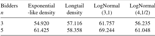
Table 1. Proportion (%) ofρin HT withu(0,·)> u(ρ,·)
Bidders Exponential Longtail LogNormal LogNormal
n -like density density (3,1) (4,1/2)
3 54.920 57.116 61.757 56.235
5 61.425 58.358 69.244 61.048
NOTE: The table shows the proportion of reserve prices in the HT set associated with revenues that are lower than the revenue at zero reserve price. For example, when values are distributed as the Longtail density and there are three bidders, 55% of the HT set produces lower revenues than zero reserve price.
seller should behave as if there will be two bidders while treating the transaction price as the highest value.
Finally, the article considers auctions with correlated val-ues (with a known number of bidders). Then, as long as the transaction price is equal to the second highest value, an assump-tion used by Aradillas-Lopez, Gandhi, and Quint (in press), the main result of the article holds, irrespective of the correlation structure.
This article is related to some other papers that have used the maxmin criterion for robust decision in various problems with partial identification such as Manski (2000), Kitagawa (2011), Menzel (2011), and Song (2012). This article also has the same spirit as Handel, Misra, and Roberts (2013) that studied demand assessment and subsequent pricing problem for a firm using the minmax-regret criterion.
The next section describes the seller’s problem and Section3 develops an optimal decision rule. Section4shows Monte Carlo experiments followed by some extensions in Section5. Section6 concludes and an appendix collects all computational details.
2. AUCTION MODELS
A single indivisible object is auctioned among n≥2 risk neutral bidders in an English auction. Each bidderiobserves only his valuevi ≥0. Assume v1, . . . , vn are drawn indepen-dently from an identical, absolutely continuous distributionPv with densitypv. LetP
j:n v andp
j:n
v be the cdf and the pdf of the jth highest order statistics among theniid values, respectively. The auction starts at zero price and at each time bidders raise the standing price ˜yby at least, the minimum bid increment. Bidding more than ˜y+is known as jump bidding. When no bidder is willing to raise ˜yfurther, the auction allocates the ob-ject to the bidder who offers the final bid at the transaction price
y:=y˜. This article makes the assumption:
Assumption 1. (A-HT) The transaction price y ≤x :=
max{v1, . . . , vn}.
This assumption is weaker than the assumptions in HT, which also require that the bidders do not let their opponents win at a price they can overbid. The datazTavailable to the seller consist of iid transaction prices (y1, . . . , yT) from pastTauctions, each withn bidders. Only the transaction prices are used because many public auctions reveal only the transaction prices and even when all bids are observed, it is not obvious that the losing bids convey any useful information when >0 or when there is jump bidding (see Lu and Perrigne2008; Quint2008; Aradillas-Lopez, Gandhi, and Quintin press).
Now, consider a seller with datazT who wishes to choose a reserve price to maximize his revenue in a future auction where
the valuation distribution remains unchanged. The future auction can take any of the “standard” auctions—a standard auction is an auction where the highest bidder gets the object. Furthermore, in line with the literature, the article also assumes that if a bidder’s value is zero, he expects to pay zero. Myerson (1981) and Riley and Samuelson (1981) showed that when the seller’s values are zero, the reserve priceρthat maximizes the revenue,
u(Pv, ρ) :=
∞
0
max{ρ, ξ}dPvn−1:n(ξ)−ρPvn:n(ρ) (1)
solves the following first-order necessary condition:
ρ=1−Pv(ρ)
pv(ρ)
. (2)
Since the seller does not know Pv, he or she cannot use Equation (2) to determineρ. For this problem, Paarsch (1997) proposed to estimatePvby treating the observed bids as losers values in the button auction model, and used the point estimates in Equation (2) instead of Pv (a.k.a. “plug-in” method). For nonparametric identification of the button auction model, see Athey and Haile (2002). When >0 or when there is jump bidding, however, the assumption that bids equal values can be unreasonable. HT show that this assumption can cause a significant bias in the estimation of Pv even for a correctly specified parametric model.
For this reason, HT only assume that bidders do not overbid their value and do not let the auction terminate at a price that they can profitably overbid. Then, HT partially identifiePvand construct a set estimator for the RMRP. These set estimates are robust to any misspecification on bidding behavior with jump bidding and >0.
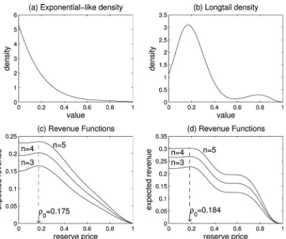
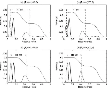
The HT interval itself, however, does not completely solve the seller’s problem. Moreover, the HT interval includes many reserve prices with revenue lower than with zero reserve price. Table 1shows that such reserve prices are about 55% to 69% of the HT intervals, each of which is obtained from bid samples of 200 auctions generated from a fixed data-generating pro-cess (DGP), that is, a combination of a valuation distribution in Figures1and2andn∈ {3,5}bidders (see sec.4for detail). In most cases, zero reserve price produces substantially higher rev-enues than average revrev-enues of the HT intervals (seeTable 2). This stems from the asymmetric shape of the revenue function. The revenue gradually increases up to the RMRP, but it drops sharply thereafter, while the upper limit of the HT interval is much higher than the RMRP (see Figures1and2).
What should then be the criteria to choose one RMRP from this interval? The next section proposes a solution to this question.
Table 2. Percentage revenue gains ofρ=0
Bidders Exponential Longtail LogNormal LogNormal
n -like density density (3,1) (4,1/2)
3 14.487 (7.483) 13.129 (8.018) 15.850 (11.486) 7.661 (1.370) 5 12.370 (5.734) 6.210 (1.388) 13.521 (8.823) 3.473 (0.388)
NOTE: The table compares the average revenue (the revenue at the midpoint) of the HT set and the revenues at zero reserve price. For example, when values are distributed as the Longtail density and there are three bidders, using zero reserve price would give revenues that are 13% (8%) higher than a reserve price randomly drawn from the HT set (the midpoint of the HT set).
Figure 1. Valuation densities and revenue functions. Panels (a) and (c) plot the exponential-like density function and associated revenue functions for alternative number of biddersn. Panels (b) and (d) similarly for the longtail values density. On panels (c) and (d),ρ0indicates the
revenue maximizing reserve price.
3. Ŵ-MAXMIN SOLUTION
The goal of this section is to develop a statistical decision method that exploits no information on bidding behavior other than the no-overbidding assumption (A-HT). That is, the method models the seller as agnostic across all possible beliefs on bid-ding behaviors as long as (A-HT) is satisfied. To this end, we employs the framework of GS because it is a parsimonious framework to represent the seller’s attitude toward the am-biguous feature of the model. Typically, other decision criteria require additional assumptions on the seller’s preference and be-liefs, which is elaborated at the end of this section. This section begins by assuming that
Assumption 2. (A-GS) The seller satisfies the axioms (A.1– A.6) in GS.
(A-GS) coincides with axioms in the classic expected utility theory, except it allows the seller to weakly prefer any convex combination of indifferent lotteries to each individual one in-stead of restricting the combination to be indifferent—ambiguity aversion, and uses a weaker version of independence. Then, GS showed that these axioms are necessary and sufficient for a de-cision maker to have a unique set of distributions and prefer an actionatobif and only if the minimal expected utility over all distributions in the set underais at least as big as underb.
To formulate the seller’s problem within this framework, the article considers the parameter vector that indexes Pv as the random vector that affects the revenue. This parameter vector is divided into two groups: identified and unidentified. The former,
θ∈, indexes the distribution of the transaction price y, that is, Py(y|θ), and the latter, h∈H, captures any discrepancy between the distributions ofyandx =max(v1, . . . , vn), so that
Py(y|θ)=Pvn:n(y|θ,0) (3)
asPx(·|θ, h)=Pvn:n(·|θ, h). Therefore, his inherently infinite dimensional, and the statistical modelPv(·|θ, h) is nonparamet-ric if θ is also infinite dimensional, or it is semiparametric, otherwise. (In the statistical decision theory, the term “param-eter” refers to the state of world, but does not suggest that the statistical model is indexed by a finite dimensional parameter.)
The article uses this configuration of parameters, so thath solely captures the lack of identification because it simplifies the way the seller’s decision process is framed. Here,h is a nuisance parameter that is related to the equilibrium bidding strategy. For example, the button auction model corresponds to a dogmatic prior onhthat puts probability one onh∗ such thatPy(·|θ)=Pvn−1:n(·|θ, h
∗). One may also put probability 1
on a differenth∗ if he believes that a different bidding model generates the data. Or, he may have a nondegenerate prior onh
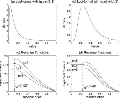
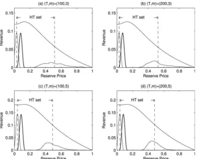
Figure 2. Valuation densities and revenue functions. Panels (a) and (c) plot the lognormal density with (μ, σ)=(3,1) and associated revenue functions for alternative number of biddersm. Panels (b) and (d) similarly for (μ, σ)=(4,1/2). On panels (c) and (d),ρ0indicates the revenue
maximizing reserve price.
reflecting his (dispersed) beliefs. Any hypothesis on bidding be-havior is, however, not verified by the datazT :=(y1, . . . , yT). Therefore, the prior on h may have a persistent influence on decision making.
To see this, suppose that the seller has the sample zT as well as a priorpθ,h over ×H. For this case, Kim (2013b) posited choosing a reserve price as the seller’s decision problem under parameter uncertainty. The article argues that if the seller behaves rationally in the sense of Savage (1954) and Anscombe and Aumann (1963), he or she would maximize the expected revenue given by
E[u(θ, h, ρ)|zT;ph]
:=
H
u(θ, h, ρ)pθ,h(θ, h|zT;ph)dhdθ, (4)
whereu(θ, h, ρ) :=u[Pv(·|θ, h), ρ] from Equation (1) and the posterior density can be obtained via Bayes’ theorem,
pθ,h(θ, h|zT;ph) :=
pθ,h(θ, h) T
t=1py(yt|θ)
pθ,h(θ, h)Tt=1py(yt|θ)dhdθ
. (5)
Kim (2013b) discussed the optimality of this Bayesian approach from the frequentist perspective, and shows that it can produce substantially higher revenues than the plug-in rule. Note,
how-ever, that since
pθ,h(θ, h|zT;ph)=ph(h|θ)
pθ(θ) T
t=1py(yt|θ)
pθ(θ)Tt=1py(yt|θ)dθ
=ph(h|θ)pθ(θ|zT),
the samplezT directly affectsθbut noth. Therefore, the impact ofph(·|θ) on the solution to maximize Equation (4) would not disappear even whenTis large.
The article takes the framework of GS to handle the ambiguity aboutph(·|·). A conditional priorph(·|θ) is said to bereasonable in this article if it conforms to (A-HT) for everyθ∈. LetŴbe the set of all priorsph(·|·) such that, for every (θ, h)∈×H
pθ(θ)ph(h|θ)>0⇔Px(ξ|θ, h)≤Py(ξ|θ), ∀ξ ∈R. (6)
Under GS, the seller considers every element inŴas equally reasonable and solves
max ρ∈Apminh∈Ŵ
E[u(θ, h, ρ)|zT;ph]. (7)
That is, the seller should choose a reserve price that maximizes the revenue in Equation (4) with respect to the most pessimistic prior inŴ.
Definition 1. A decision rule that solves Equation (7) for every realization ofzT is called theŴ-maxmin rule.
For an intuitive interpretation of theŴ-maxmin rule, suppose the seller consults with many experts about the bidding behavior, that is,h, each proposing a different, but reasonable opinion. Then, the Ŵ-maxmin criterion implies that the seller should take the most pessimistic prediction about the revenue to secure against the worst possible outcomes.
TheŴ-maxmin rule is robust to the choice of prior over the unidentified parameter. Usually, solving Equation (7) is com-putationally expensive because the “min” part solves an opti-mization problem over a space of high-dimensional functions for everyρ. This issue does not, however, arise for the seller’s problem as the minimization part has a simple solution, as shown below.
Proposition 1. Let the setŴsatisfy the property (6). Under (A-HT) and (A-GS),
for anyj ≤n (Lemma 1, HT). Then, using the inequality for
j =n−1 gives
Intuitively, suppose there are two valuation distributions, one first-order stochastically dominating the other. Then, the revenue under the latter is smaller for everyρ. The proposition simply shows that the valuation distribution whose highest order statis-tics equals yis dominated by all other valuation distributions that are “reasonable” with respect to (A-HT). It is, therefore, associated with the smallest revenue. This result implies that choosing the worst prior amounts to treatingyasx.
Until now, the article has assumed that the number of bid-ders is known. How should a seller choose a reserve price if it is also ambiguous? This article considers two subcases: (i) only the number of bidders in future (T +1)th-auction,nT+1,
is ambiguous, and (ii) the number of bidders in the past and fu-ture auctions is equal but ambiguous, that is an unknown n is constant across all t =1, . . . , T +1 auctions. Let the util-ity be indexed by n, that is, u(θ, h, ρ;n). For the case (i),
the posterior expectation of the revenue in Equation (4) can be obtained as before and the worst case for the seller is that the transaction price is generated from auctions with two bidders.
Some additional notations are required: letN := {2, . . . ,n¯} with ¯n <∞ be the set of all possible number of bidders, and let Ŵ′ be the set of all joint priors ph,nT+1(·,·|θ) over
H×Nthat satisfy (A-HT), that is,pθ(θ)ph,n
T+1(h, n|θ)>0⇔
Px(ξ|θ, h, n)≤Py(ξ|θ, n), wherePx(·|θ, h, n) is the cdf of the highest order statistics of a random sample of values of sizen andPy(·|θ, n) is the cdf of the transaction price of auctions with nbidders.
Corollary 1. Under (A-HT) and (A-GS), and uncertainty aboutnT+1∈N
est order statistics amongniid draws fromF(·). The fact that
F(n−1:n)(x)≥F(n:n+1)(x) for allx ∈ ℜfollows from
2. Back to the problem, the seller is uncertain about two pa-rameters ˜n:=nT+1andh. Following the same argument as in
where the last inequality is due to inequality shown above. More-over, for any ρ∈A⊂ ℜ+, ρPn˜: ˜n
Thus, theŴ-maxmin rule says when the seller is ambiguous aboutnT+1, he should believe that there will be only two bidders,
that isnT+1=2. It is intuitive that since the competition with
two bidders is the lowest, the revenue from two bidder auctions is the smallest, if all else is equal.
Consider now the case (ii) where the ambiguousnis constant across auctions. By Proposition 1, for a fixedn∈N, the lowest posterior expectation of the revenue can be written as
En[u(θ, hn, ρ;n)|zT, δhn]
but sincenis ambiguous, theŴ-maxmin rule solves
max
ρ∈Aminn∈NEn[u(θ, hn, ρ;n)|zT, δhn].
Note thatnnow affects bothu(·) and the posterior, and the rule maximizes the lower envelop of the ¯nposterior expectations of the revenue, each with a differentn∈N.
This section concludes with a brief discussion about a few widely used alternative decision criteria. As noted earlier, the pure Bayesian decision rule can be sensitive to the choice of the prior, which motivates the use of theŴ-maxmin criteria. One could employ theŴ-maxmin regret rule, instead. It is, how-ever, just theŴ-maxmin rule with a modified utility function,
˜
u(θ, h, ρ) :=u(θ, h, ρ)−maxρ˜u(θ, h,ρ˜). But, this
modifica-tion lacks an economic interpretamodifica-tion. Moreover, in general, such a modification is used when the original (usually, some maxmin) rule exhibits an odd behavior because the worst sce-nario is extremely unreasonable (see sec. 5.5; Berger 1985). But, theŴ-maxmin rule does not have this problem because the worst prior is already reasonable, by construction. The multiplier preferences of Hansen and Sargent (2001) are also an alterna-tive decision criterion. Its optimal decision rule is equivalent to a Bayesian decision rule with an initial prior and a modified utility function (see also Strazalecki2011). This modification, however, depends on the decision maker’s confidence about the initial prior. Thus, the criterion can be used only under an ar-bitrary assumption about the initial prior and the confidence, which is against the spirit of the article to not use any informa-tion on bidding behavior other than (A-HT). One could also use thesecond-order probabilitymodel of Klibanoff, Marinacci, and
Mukerji (2005), but that too requires unverifiable assumptions about the second-order priors and the utility function.
4. COMPARISONS BETWEENŴ-MAXMIN AND HT
This section investigates the performance of theŴ-maxmin rule viz-a-viz the true RMRP’s and the HT interval for four different valuation densities. The densities and the associated revenue functions are shown in Figures1 and2 forn bidders withn∈ {3,4,5}.Figure 1is associated with the density similar to that of an exponential distribution and a long-tailed density, andFigure 2 is associated with lognormal densities with dif-ferent parameters; see Appendix A for construction of these density functions. (Notice that the revenue structures here are all asymmetric, so that the cost of choosingρ > ρ0is more than
choosingρ < ρ0for the same magnitude of bias.)
For each of these valuation densities, the experiments con-sider (n, T)∈ {3,5} × {100,200}leading to a total of 16 ex-periments. Each experiment, that is, each triplet of (Pv, n, T), conducts 1000 Monte Carlo replications. For each experiment, the seller randomly selects a bidder and usesy˜ :=0.05×y˜
as the minimum bid increment rule. The chosen bidder bids exactly ˜y+y˜, as long as it is less than his or her value (no
jump bidding). Each replication usesonlytransaction prices to implement alternative decision rules: (i) the rule that randomly chooses a point from the HT interval, HTRAN, (ii) the rule that
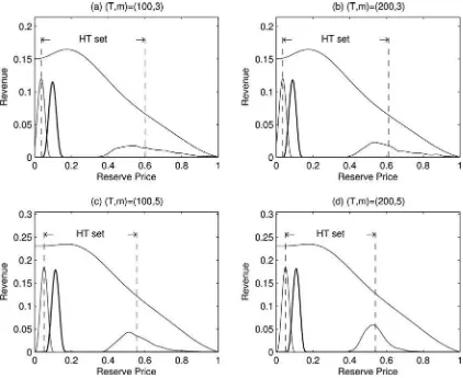
Figure 3. Exponential-like distribution. The revenue function is plotted along with the distributions of the lower and the upper bounds for the HT set (light lines) and the reserve prices chosen by theŴ-maxmin (heavy).
chooses the midpoint of the HT interval, HTMID, and (iii) the
rule that chooses the true RMRP, Oracle. The comparison with Oracle provides valuable information about how closely the
Ŵ-maxmin rules approximate the true optimal revenue. LetD collect these three rules.
For the implementation of theŴ-maxmin rules, the experi-ments specify the distribution of the transaction price using the Bernstein cdf:
Py(y|θ)=
⎡
⎣
k
j=1
θjBeta(y|j, k−j+1)
⎤
⎦
n
, (10)
where θ∈k−1, the k−1 dimensional unit simplex, that
is, θj ≥0 for all j =1, . . . , k−1 and k−j=11θj ≤1, and Beta(·|a, b) denotes the beta cdf with parametersaandb; see (Petrone 1999a,b) for a nonparametric Bayesian method that uses the beta mixture. This article employs the model with
k=15 with the uniform prior over14. AppendixAprovides
some information on the flexibility of the model.
Each Monte Carlo replication q=1, . . . ,1000 simulates a samplezqT, and implements every decision rule inD. Letρdq be the reserve price chosen by the ruled ∈D, and letuqd be the true revenue atρdq, that is,uqd :=u(Pv, ρdq). Then, the percentage revenue gains of theŴ-maxmin approach over alternative rules
are computed by
1 1000
1000
q=1 uq
Ŵ−u q d
uqd
×100% (11)
ford ∈ {HTRAN,HTMID,Oracle}.
Table 3shows the results. For each (Pv, n, T), columns (I), (I I), and (I I I) are the percentage revenue gains (11) of the
Ŵ-maxmin rule relative to HTRAN, HTMID, and Oracle,
respec-tively. For example, the first row and column (I) is associated with (Pv, n, T)=(exponential-like,3,100). It shows that the revenue gain of the Ŵ-maxmin approach over the overall HT interval is around 23.64%. WithT =200, this gain is around 23.62% (second row). The third and fourth rows collect the results whenn=5. When HTMIDis considered, theŴ-maxmin
rule still produces substantially larger revenues (7%–15%; see columnI I). Moreover, the loss ofŴ-maxmin relative to the true RMRP is relatively small (see columnI I I).
Figure 3 explains the revenue gains. Each panel depicts the (simulated) distribution of reserve prices chosen underŴ -maxmin rule (heavy solid) and the lower and upper bounds for the HT interval (light solid) along with the revenue function. The left (right) panels are withT =100 (T =200), and the upper (the lower) panels are withn=3 (n=5). The left-upper panel shows that the upper bound of the HT interval is distributed around 0.6 with a wide support, while the revenue function
Figure 4. Longtail distribution. The revenue function is plotted along with the distributions of the lower and the upper bounds for the HT set (light lines) and the reserve prices chosen by theŴ-maxmin (heavy).
Table 3. Percentage revenue gain of theŴ-maxmin rule
HTRAN HTMID Oracle
Pv n T (I) (I I) (I I I)
Exponential 3 100 23.640 15.116 −3.933 200 23.619 14.912 −4.618 5 100 17.079 9.062 −0.854 200 15.230 7.081 −0.934 Longtail 3 100 19.343 16.152 −1.265 200 17.767 13.072 −1.420 5 100 8.279 3.339 −0.139 200 6.798 1.575 −0.149 LogN(3,1) 3 100 23.785 18.317 −2.105 200 24.077 18.586 −2.652 5 100 17.727 11.911 −0.497 200 16.549 10.533 −0.562 LogN(4,1/2) 3 100 9.643 2.185 −0.330 200 8.606 1.641 −0.373 5 100 4.380 0.570 −0.013 200 3.623 0.401 −0.015 NOTE: This table compares the performance ofŴ-maxmin rule and the rules using the HT interval. For example, for (Pv, n, T)=(exponential,3,100), theŴ-maxmin rule with
nknown produces 23.64% higher revenues than a randomly chosen reserve price from the HT interval (see column I).
indicates that all the reserve prices larger than approximately 0.3 produces lower revenues than zero reserve price. This im-plies that a significant portion (54.92%; Table 1) of the HT interval is less profitable than zero reserve price. On the other
hand, theŴ-maxmin rule is distributed over the area in which the revenue is increasing, selecting higher reserve prices than the lower bound of the HT interval. As a result, theŴ-maxmin rule produces larger revenues than HTRANand HTMID.
The revenue comparisons for other valuation densities are similar: see the rest of the table and see also Figures3–6. In con-clusion, the simulation results here suggest that theŴ-maxmin approach can provide a practical policy recommendation.
5. SOME EXTENSIONS
This section extends the Ŵ-maxmin framework to auctions with correlated values, auctions with binding reserve price, and auctions with observed covariates.
5.1 Correlated Private Values
This subsection considers English auctions with correlated private values as in Aradillas-Lopez, Gandhi, and Quint (in press). While the environment and the data structure are the same as before, let the bidders’ value (v1, . . . , vn) be jointly distributed asPv(·, . . . ,·|θ, h). Since the revenue function is still given by Equation (1), the choice of a reserve price depends on the distributions of the second highest valuePn−1:n
v (·|θ, h) and the highest valuePn:n
v (·|θ, h). But unlike IPV, when values are
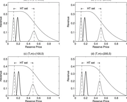
Figure 5. Lognormal (3,1). The revenue function is plotted along with the distributions of the lower and the upper bounds for the HT set (light lines) and the reserve prices chosen by theŴ-maxmin (heavy).
Figure 6. Lognormal (4,1/2). The revenue function is plotted along with the distributions of the lower and the upper bounds for the HT set (light lines) and the reserve prices chosen by theŴ-maxmin (heavy).
correlated, the distributions of order statistics are not necessarily linked through the identical marginal valuation distribution. In particular, Equation (9) does not hold anymore. Thus, following Aradillas-Lopez, Gandhi, and Quint (in press), it is assumed that
Assumption 3. (A-AGQ) The transaction price is equal to the second highest value.
Under (A-AGQ), zT point identifies Pvn−1:n(·|θ, h), that is,
Py(·|θ)=Pvn−1:n(·|θ, h). Using Px(·|θ, h)=Pvn:n(·|θ, h), the revenue function (1) is written as
u(θ, h, ρ)= ∞
0
max{ρ, ξ}dPy(ξ|θ)−ρPx(ρ|θ, h).
Since Px(·|θ, h)=Pvn:n(·|θ, h)≤Pvn−1:n(·|θ, h)=Py(·|θ) and
Py(ξ|θ)=Pvn:n(·|θ,0) for all θ,ρ, and h, it follows that the revenue is bounded below by u(θ,0, ρ), that is, u(θ, h, ρ)≥
u(θ,0, ρ). In other words, the worst case is whenh=0 and hence the seller should still solve Equation (8).
Proposition 2. Let the setŴsatisfy the property (6). When the values are correlated, under (A-GS) and (A-AGQ), Equation (8) holds.
Hence, Proposition 2 implies that when the distribution of the second highest value is identified by the transaction pricey, it
is still optimal to treatyasx, the highest value for choosing a reserve price.
5.2 Binding Reserve Prices
Back to the IPV case. Suppose the datazT contains a bind-ing reserve priceρ1, that is, Pv(ρ1|θ, h)>0. Then, the seller observes transaction prices only if there isi∈ {1, . . . , n}such thatvi ≥ρ1. Lemma 5 of HT shows that as long asρ1< ρ0 :=
arg maxρu(θ, h, ρ), and u(θ, h, ρ) is strictly pseudo-concave inρ, the RMRP with the truncated distribution ˜Pv(v|θ, h) := [Pv(v|θ, h)−Pv(ρ1|θ, h)]/[1−Pv(ρ1|θ, h)] equals the RMRP
associated with the original distributionPv(v|θ, h). Therefore, Proposition 1 and Corollary 1 hold with ˜Pv(v|θ, h) instead of
Pv(v|θ, h).
Whetherρ1< ρor not is an empirical question. The empirical
literature has commonly found that the actual reserve prices are very small for many important public auctions. For example, see Paarsch (1997) for the British Columbia Timber sales and Haile and Tamer (2003) and Lu and Perrigne (2008) for the U.S. timber sales. Those timber auctions set reserve prices following some simple rule of thumb, which is a function of some observed characteristics such as the experts’ estimate of the market value and total volume of timbers. Since the literature testifies that the actual reserve prices are too small to be optimal, those rules
may be regarded as some random rule from a formal decision perspective.
5.3 Auction Specific Covariates
Many datasets provide the information on auction specific characteristics,ωt. This subsection discusses the extension of theŴ-maxmin rule to situations where the valuation distribution depends onωt. The stochastic dominance relation in Proposition 1 and Corollary 1 still holds for the (conditional) valuation distributionPv(·|θ, h, ω) for a givenω, and the lowest revenue is attained ath=0. Hence, theŴ-maxmin approach is applicable with the observed characteristics for the future auction, that is,
ωT+1.
To implement theŴ-maxmin rule, therefore, it is sufficient to model the valuation distributionPvunder the worst prior onh, that is,
Py(y|θ, ω)=[Pv(y|θ, h=0, ω)]n,
where the left-hand side is the cdf of the observed transaction price, which is equal to the cdf of the highest value on the right-hand side withh=0. One way to specify it would be as follows. LetQ(·|γ) be a parametric distribution on the support of the value that approximates the valuation distribution and(·|ψ) be a flexible (or nonparametric) distribution defined on [0,1]. For example, could be modeled by a series representation such as the Bernstein polynomial distribution in Equation (10). Then, it can be specified as
Pv(v|θ, h=0) :=[Q(v|γ)|ψ]
withθ :=(γ , ψ). Note thatQapproximates the valuation distri-bution first andHimproves the approximation (under the worst prior onh).
If each auction is characterized byωt, one may model the parameter γ as a function of ωt ∈ ℜd. That is, the
distribu-The problem of choosing a reserve price using a bid sam-ple has been widely studied in the auction literature, since Paarsch (1997). This article proposes to use decision making under ambiguity to determine a reserve price when a sample of transaction prices from English auctions does not point-identify the valuation distribution and the seller is unwilling to make strong (unverifiable) bidding assumptions other than bidders never overbidding.
This article extends Kim (2013b) to the partially identified auction models of HT, and proposes to use the maxmin decision criteria axiomatized by Gilboa and Schmeidler (1989), where the seller in the face of ambiguity chooses a reserve price that maximizes the worst case revenue. Under the only behavioral assumption of no-overbidding, this article shows that it is op-timal to employ the Bayesian decision rule of Kim (2013b) interpreting the transaction prices as the highest value. A Monte Carlo exercise shows that this procedure performs well.
Exten-sions to auctions with uncertain number of bidders, correlated values, binding reserve prices, and observed characteristics are also considered.
For the IPV case, this article abstracts away the choice of auction format on account of the revenue equivalence theorem, and for the correlated values, it implicitly assumes the seller uses the English auction as it gives higher revenues than the first price auction (see Milgrom and Weber 1982). However, if bidders are asymmetric, neither the revenue equivalence theorem nor the revenue ranking holds even when values are independent (see Marshall et al. 1994; Maskin and Riley2000; Cantillon 2008). Hence, the choice of auction format is also an important issue. For this reason, this article does not pursue the case of asymmetric bidders, but a few words on it are in order.
If the format is fixed to be the English auction, theŴ-maxmin procedure can be applied to auctions with the asymmetric bidders under some assumptions. For example, if bidders are grouped by different types and the probability for each type is known, then it is still optimal for the seller to treat the trans-action prices as the valuation and compute the optimal reserve price with respect to the mixture distribution, where the mix-ing weights can be identified from the data. In the U.S. timber auctions, for example, information on the fractions for small mills or huge mills is available. Similarly, the bidding history of highway procurements reveals the types of large companies and small local companies.
To sum up, this article takes a first step for empirical auction design where the structural parameter is partially identified, by proposing a method that is decision theoretically well-founded, simple, and profitable. A further investigation for more general situations including auctions with asymmetric bidders would be important future research.
APPENDIX A: VALUATION DENSITIES AND FLEXIBILITY OF THE BERNSTEIN DENSITY
A.1 Construction of True Valuation Densities
Figure 1is associated with the density similar to that of an ex-ponential distribution and a long-tailed density. These densities have the form of Equation (10) withk=15. For the exponential-like density, the parameter values are θ:=(0.3548, 0.2350, 0.1486, 0.0946, 0.0466, 0.0440, 0.0217, 0.0119, 0.0089, 0.0080, 0.0084, 0.0081, 0.0049, 0.0028, 0.0017) and for the long-tailed density,θ:=(0.0748, 0.1403, 0.1871, 0.5145, 0.0009, 0.0009, 0.0009, 0.0009, 0.0009, 0.0009, 0.0009, 0.0750, 0.0009, 0.0009, 0.0002). Similarly,Figure 2is associated with lognormal densi-ties with different parameters. The lognormal distributions with (μ, σ)=(3,1) and (4,1/2) are truncated at the 99th percentile and rescaled, so that their supports are the unit interval. HT employed the lognormal densities that appear inFigure 2for Monte Carlo studies.
A.2. Flexibility of the Bernstein Density
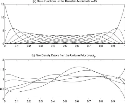
Figure 7gives some information on the flexibility of the BPD in Equation (10) withk=15. Panel (a) plots 15 beta density functions (basis functions for the model) and panel (b) plots five valuation densities that are drawn from the uniform prior over
Figure 7. Bernstein density withk=15. This figure gives some information on how flexible the Bernstein density model withk=1 would be. Panel (a) plots 15 basis functions and panel (b) plots five densities drawn from a uniform prior over14.
14, that is, each of the five curves on panel (b) is a mixture of
the 15 beta densities on panel (a).
APPENDIX B: COMPUTATION
As mentioned in Section4, there are 16 experiments. Each experiment employs 1000 Monte Carlo replication to make a long-run comparison between theŴ-maxmin approach and the average performance of the HT interval. The first replication employs the Adaptive Metropolis (AM) algorithm of Haario, Saksman, and Tamminen (2001) to draw{θs}Ss=1from the pos-terior distribution, and all other replications q =2, . . . ,1000 employ the importance sampling using the{θs}Ss=1from the first replication and the new datazqT.
B.1 Sampling from the Posterior with a Flat Prior: 1st Replication
Letz1
T :=(y11, . . . , yT1) denote the simulated auction data of sizeTin the first Monte Carlo replication;q =1. Let alsoθ0:=
(1k, . . . ,1k)(k−1)×1be the initial vector for the AM algorithm. At
eachs=1, . . . , S, a candidate parameter vector is drawn from ˜
θ|θ0, θ1, . . . , θs−1 ∼N(θs−1, (θ0, θ1, . . . , θs−1)),
where N(a, b) is the k−1 dimensional multivariate normal distribution with mean vector aand covariance matrix b, and
fors <50,
(θ0, θ1, . . . , θs−1) :=
2.382
k−1
Ik−1
withIk−1being thek−1 dimensional identity matrix, but for
s≥50,
(θ0, θ1, . . . , θs−1)
:= ⎧ ⎪ ⎨
⎪ ⎩
2.382
k−1
Ik−1 with probability 0.05
cov(θ0, θ1, . . . , θs−1) with probability 0.95,
where cov(a1, . . . , an) denotes the sample covariance matrix of nvectorsa1, . . . , an. Then, letθs :=θ˜with probability
α( ˜θ , θ0, . . . , θs−1)=min
1,I
k−1( ˜θ)· T
t=1
py(yt1|θ˜)
py(yt1|θs−1)
,
(B.1)
or letθs :=θs−1with probability 1−α( ˜θ , θ0, . . . , θs−1). Note that since the uniform prior is employed, the prior ratio inα(·) reduces to the indicator for the k−1 dimensional simplex, I
k−1(·).
The likelihood can be evaluated as follows: letxbe a col-umn vector ofN numbers in [0,1], and letBk(x) be aN×k matrix with the (i, j)th element being beta(xi|j, k−j+1), for
example, ifk=15, b. Similarly, defineCk(x) with the cdf’s instead of pdf’s, for example, ifk=15, In addition, let ιT be the T-dimensional column vector of ones. Let ¯×denote the element-wise multiplication operator, for example, (a1, a2) ¯×(b1, b2)=(a1b1, a2b2). Define
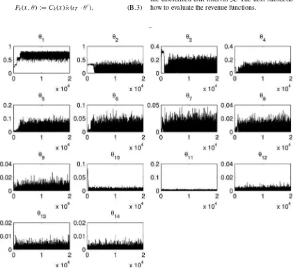
Each experiment iterates the AM algorithm 20,000,000 times, recording every 1000th iteration. Figure 8 shows the mix-ing quality of the MCMC traces for each parameters for the experiment (Pv, T , m)=(exponential-like,100,3). The first half of the outcomes is discarded as a burn-in phase. Thus, the experiment employsS=10,000 draws from the posterior to implement theŴ-maxmin rule.
In particular, theŴ-maximin rule solves
max
j/1000. The revenueuis computed via the trapezoid rule over the discretized unit interval A. The next subsection describes how to evaluate the revenue functions.
Figure 8. MCMC outcomes: exponential-like, (T , m)=(100,3). The figure shows the MCMC outcomes for each parameter θj with
j=1, . . . ,14 for the experiment with the exponential-like valuation density and (T , m)=(100,3). Each panel records every 1000th iteration from 20,000,000 AM outcomes. The MCMC outcomes for other experiments are similar to the ones here.
B.2. Evaluation of the Revenue Functions
The seller’s revenue in Equation (1) can be written as
u(θ,0, ρ;m)
The trapezoid rule approximates all the integrals of Equation (B.5) using the J =1001 equidistant reference points on the unit interval,A.
respectively. They are the 1001 dimensional column vectors of pdf’s and cdf’s evaluated at eachx ∈A. It is straightforward to compute the first term of Equation (B.5). Finally, let
D1 :=
B.3. Replications 2 to 1000: Importance Sampling
LetzqT :=(y11, . . . , yT1) denote the simulated auction data of sizeTin theqth Monte Carlo replication withq=2, . . . ,1000. Using importance sampling method withθ1, . . . , θS from the first replication, it is possible to approximate the revenue for each point inA. In particular, let
ωq(θs) :=
The authors thank Keisuke Hirano, Aleksey Tetenov, Amit Gandhi, Laurent Lamy, Myoung-jae Lee, and seminar audience at Universities of Auckland, Chicago, and Queensland, and at the 4th World Congress of the Game Theory Society. The au-thors thank the referee and the associate editor for useful and insightful suggestions, which improved the quality and the scope of the article. Kim acknowledges the financial support from the Faculty of Business Research Grant, UTS.
[Received June 2012. Revised January 2013.]
REFERENCES
Anscombe, F. J., and Aumann, R. J. (1963), “A Definition of Subjective Proba-bility,”Annals of Mathematical Statistics, 34, 199–205. [387]
Aradillas-Lopez, A., Gandhi, A., and Quint, D. (in press), “Identification and Testing in Ascending Auctions With Unobserved Heterogeneity,” Econo-metrica. [385,391]
Athey, S., and Haile, P. A. (2002), “Identification of Standard Auction Models,”
Econometrica, 70, 2107–2140. [384,385]
Berger, J. O. (1985), Statistical Decision Theory and Bayesian Analysis, Springer Series in Statistics, New York: Springer. [389]
Cantillon, E. (2008), “The Effect of Bidders Asymmetries on Expected Revenue in Auctions,”Games and Economic Behavior, 62, 1–25. [393]
Gilboa, I., and Schmeidler, D. (1989), “Maxmin Expected Utility With Non-Unique Prior,”Journal of Mathematical Economics, 18, 141–153. [384,393] Haario, H., Saksman, E., and Tamminen, J. (2001), “An Adaptive Metropolis
Algorithm,”Bernoulli, 7, 223–242. [394]
Haile, P. A., and Tamer, E. (2003), “Inference With an Incomplete Model of English Auctions,”Journal of Political Economy, 111, 1–51. [384,392] Handel, B. R., Misra, K., and Roberts, J. W. (2013), “Robust Firm Pricing With
Panel Data,”Journal of Econometrics, 174, 165–185. [385]
Hansen, L. P., and Sargent, T. J. (2001), “Robust Control and Model Uncer-tainty,”American Economic Review, Papers and Proceedings, 91, 60–66. [389]
Harris, M., and Raviv, A. (1981), “Allocation Mechanisms and the Design of Auctions,”Econometrica, 49, 1477–1499. [384]
Kim, D.-H. (2013a), “Flexible Bayesian Analysis of First Price Auctions Using a Simulated Likelihood,” Mimeo. [384]
——— (2013b), “Optimal Choice of a Reserve Price under Uncertainty,” Inter-national Journal of Industrial Organization, forthcoming. [384,387,393] Kitagawa, T. (2011), “Intersection Bounds, Robust Bayes, and Updating
Am-biguous Beliefs,” Mimeo. [385]
Klibanoff, P., Marinacci, M., and Mukerji, S. (2005), “A Smooth Model of Decision Making Under Ambiguity,”Econometrica, 73, 1849–1892. [389] Krasnokutskaya, E. (2011), “Identification and Estimation of Auction Models
With Unobserved Heterogeneity,”Review of Economic Studies, 78, 293– 327. [384]
Li, T., Perrigne, I., and Vuong, Q. (2003), “Semiparametric Estimation of the Optimal Reserve Price in First-Price Auctions,”Journal of Business & Eco-nomic Statistics, 21, 53–64. [384]
Lu, J., and Perrigne, I. (2008), “Estimating Risk Aversion From Ascending and Sealed-Bid Auctions: The Case of Timber Auction Data,”Journal of Applied Econometrics, 23, 871–896. [385,392]
Manski, C. F. (2000), “Identification Problems and Decisions Under Ambigu-ity: Empirical Analysis of Treatment Response and Normative Analysis of Treatment Choice,”Journal of Econometrics, 95, 415–442. [385]
Marshall, R., Meurer, M., Richard, J., and Stromquist, W. (1994), “Numeri-cal Analysis of Asymmetric First Price Auctions,”Games and Economic Behaviour, 7, 193–220. [393]
Maskin, E., and Riley, J. (2000), “Asymmetric Auctions,”Review of Economic Studies, 67, 413–438. [393]
Menzel, K. (2011), “MCMC Methods for Incomplete Structural Models of Social Interactions,” Mimeo. [385]
Milgrom, P., and Weber, R. (1982), “A Theory of Auctions and Competitive Bidding,”Econometrica, 50, 1089–1122. [393]
Myerson, R. B. (1981), “Optimal Auction Design,”Mathematics of Operations Research, 6, 58–73. [384,385]
Paarsch, H. (1997), “Deriving an Estimate of the Optimal Reserve Price: An Application to British Columbian Timber Sales,”Journal of Econometrics, 78, 333–357. [384,385,392,393]
Petrone, S. (1999a), “Bayesian Density Estimation Using Bernstein Polynomi-als,”Canadian Journal of Statistics, 27, 105–126. [390]
——— (1999b), “Random Bernstein Polynomials,”Scandinavian Journal of Statistics, 26, 373–393. [390]
Quint, D. (2008), “Unobserved Correlation in Private-Value Ascending Auc-tions,”Economics Letters, 100, 432–434. [385]
Riley, J., and Samuelson, W. (1981), “Optimal Auctions,”American Economic Review, 71, 381–392. [384,385]
Savage, L. (1954),Foundation of Statistics, Wiley, Reissued in 1972 by New York: Dover. [387]
Song, K. (2012), “Point Decisions for Interval-Identified Parameters,” forth-coming inEconometric Theory. [385]
Strazalecki, T. (2011), “Axiomatic Foundations of Multiplier Preferences,”
Econometrica, 79, 47–73. [389]