Full Terms & Conditions of access and use can be found at
http://www.tandfonline.com/action/journalInformation?journalCode=ubes20
Download by: [Universitas Maritim Raja Ali Haji] Date: 11 January 2016, At: 19:51
Journal of Business & Economic Statistics
ISSN: 0735-0015 (Print) 1537-2707 (Online) Journal homepage: http://www.tandfonline.com/loi/ubes20
Minimum Distance Estimation of Possibly
Noninvertible Moving Average Models
Nikolay Gospodinov & Serena Ng
To cite this article: Nikolay Gospodinov & Serena Ng (2015) Minimum Distance Estimation of
Possibly Noninvertible Moving Average Models, Journal of Business & Economic Statistics, 33:3, 403-417, DOI: 10.1080/07350015.2014.955175
To link to this article: http://dx.doi.org/10.1080/07350015.2014.955175
Accepted author version posted online: 21 Aug 2014.
Submit your article to this journal
Article views: 166
View related articles
Minimum Distance Estimation of Possibly
Noninvertible Moving Average Models
Nikolay G
OSPODINOVResearch Department, Federal Reserve Bank of Atlanta, Atlanta, GA 30309 ([email protected])
Serena N
GDepartment of Economics, Columbia University, New York, NY 10027 ([email protected])
This article considers estimation of moving average (MA) models with non-Gaussian errors. Information in higher order cumulants allows identification of the parameters without imposing invertibility. By allowing for an unbounded parameter space, the generalized method of moments estimator of the MA(1) model is classical root-Tconsistent and asymptotically normal when the MA root is inside, outside, and on the unit circle. For more general models where the dependence of the cumulants on the model parameters is analytically intractable, we consider simulation-based estimators with two features. First, in addition to an autoregressive model, new auxiliary regressions that exploit information from the second and higher order moments of the data are considered. Second, the errors used to simulate the model are drawn from a flexible functional form to accommodate a large class of distributions with non-Gaussian features. The proposed simulation estimators are also asymptotically normally distributed without imposing the assumption of invertibility. In the application considered, there is overwhelming evidence of noninvertibility in the Fama-French portfolio returns.
KEY WORDS: Generalized lambda distribution; GMM; Identification; Non-Gaussian errors; Noninvert-ibility; Simulation-based estimation.
1. INTRODUCTION
Moving average (MA) models can parsimoniously charac-terize the dynamic behavior of many time series processes. The challenges in estimating MA models are twofold. First, invertible and noninvertible MA processes are observationally equivalent up to the second moments. Second, invertibility re-stricts all roots of the MA polynomial to be less than or equal to one. This upper bound renders estimators with nonnormal asymptotic distributions when some roots are on or near the unit circle. Existing estimators treat invertible and noninvertible processes separately, requiring the researcher to take a stand on the parameter space of interest. While the estimators are super-consistent under the null hypothesis of an MA unit root, their distributions are not asymptotically pivotal. To our knowledge, no estimator of the MA model exists, which achieves identifi-cation without imposing invertibility and yet enables classical inference over the whole parameter space.
Both invertible and noninvertible representations can be con-sistent with economic theory. For example, if the logarithm of asset price is the sum of a random walk component and a station-ary component, the first difference (or asset returns) is generally invertible, but noninvertibility can arise if the variance of the sta-tionary component is large. While noninvertible models are not ruled out by theory, invertibility is often assumed in empirical work because it provides the identification restrictions without which maximum likelihood and covariance structure-based es-timation of MA models would not be possible when the data are normally distributed. Invertibility can also be used to narrow the class of equivalent dynamic stochastic general equilibrium (DSGE) models, as in Komunjer and Ng (2011). Obviously, falsely assuming invertibility will yield an inferior fit of the data. It can also lead to spurious estimates of the impulse response
coefficients, which are often the objects of interest, as shown by Fern´andez-Villaverde et al. (2007) using the permanent income model. Hansen and Sargent (1991), Lippi and Reichlin (1993), and Fern´andez-Villaverde et al. (2007), among others, empha-sized the need to verify invertibility because it affects how we interpret what is recovered from the data.
While economic analysis tends to only consider parameter values consistent with invertibility, it is necessary in many sci-ence and engineering applications to admit parameter values in the noninvertible range. For example, in analysis of seismic and communication data, noninvertible filters are necessary to recover the earth’s reflectivity sequence and to back out the underlying message from a distorted one, respectively. A key finding in these studies is that higher order cumulants are nec-essary for identification of noninvertible models, implying that the assumption of Gaussian errors must be abandoned. Lii and Rosenblatt (1992) approximated the non-Gaussian likelihood of noninvertible MA models by truncating the representation of the innovations in terms of the observables. Huang and Paw-itan (2000) proposed least absolute deviations (LAD) estima-tion using a Laplace likelihood. This quasi-maximum likelihood (QML) estimator does not require the errors to be Laplace dis-tributed, but they need to have heavy tails. Andrews, Davis, and Breidt (2006,2007) considered LAD and rank-based esti-mation of all-pass models, which are special noncausal and/or noninvertible autoregressive and moving average (ARMA)
© 2015American Statistical Association Journal of Business & Economic Statistics
July 2015, Vol. 33, No. 3 DOI:10.1080/07350015.2014.955175
Color versions of one or more of the figures in the article can be found online atwww.tandfonline.com/r/jbes.
403
models in which the roots of the autoregressive polynomial are reciprocals of the roots of the MA polynomials. Meitz and Saikkonen (2011) developed maximum likelihood estimation of noninvertible ARMA models with ARCH errors. However, there exist no likelihood-based estimators that have classical properties while admitting an MA unit root in the parameter space.
This article considers estimation of MA models without im-posing invertibility. We only require that the errors are non-Gaussian but we do not need to specify the distribution. Iden-tification is achieved by the appropriate use of third and higher order cumulants. In the MA(1) case, “appropriate” means that multiple third moments are necessary, as a single third moment still does not permit identification. In general, identification of possibly noninvertible MA models requires using more uncondi-tional higher order cumulants than the number of parameters in the model. We make use of this identification result to develop generalized method of moments (GMM) estimators that are root-Tconsistent and asymptotically normal without restricting the MA roots to be strictly inside the unit circle. The estimators minimize the distance between sample-based statistics and their model-based analog. When the model-implied statistics have known functional forms, we have a classical minimum distance estimator.
A drawback of identifying the parameters from the higher order sample moments is that a long span of data is required to precisely estimate the population quantities. This issue is important because for general ARMA(p, q) models, the num-ber of cumulants that needs to be estimated can be quite large. Accordingly, we explore the potential of two simulation estima-tors in providing bias correction. The first (simulated method of moments, SMM) estimator matches the sample to the simu-lated unconditional moments as in Duffie and Singleton (1993). The second is a simulated minimum distance (SMD) estima-tor in the spirit of Gourieroux, Monfort, and Renault (1993) and Gallant and Tauchen (1996). Existing simulation estima-tors of the MA(1) model impose invertibility and therefore only need the auxiliary parameters from an autoregression to achieve identification. We show that the invertibility assumption can be relaxed but additional auxiliary parameters involving the higher order moments of the data are necessary. In the SMD case, this amounts to estimating an additional auxiliary regression with the second moment of the data as a dependent variable. An important feature of the SMM and SMD estimators is that errors with non-Gaussian features are simulated from the gener-alized lambda distribution (GLD). These two simulation-based estimators also have classical asymptotic properties regardless of whether the MA roots are inside, outside, or on the unit circle.
The article proceeds as follows. Section 2 highlights two identification problems that arise in MA models. Section 3 presents identification results based on higher order moments of the data. Section4discusses GMM estimation of the MA(1) model while Section 5 develops simulation-based estimators for more general MA models. Simulation results and an anal-ysis of the 25 Fama-French portfolio returns are provided in Section 5. Section 6 concludes. Proofs are given in the Appendix.
2. IDENTIFICATION PROBLEMS IN MODELS WITH AN MA COMPONENT
Consider the ARMA (p,q) process:
α(L)yt=θ(L)et, (1) where L is the lag operator such that Lpy
t =yt−p and the lag polynomialα(L)=1−α1L− · · · −αpLphas no common roots withθ(L)=1+θ1L+ · · · +θqLq. Here,yt can be the error of a regression model
Yt=xt′β+yt,
where Yt is the dependent variable andxt are exogenous re-gressors. In the simplest case whenxt =1,ytis the demeaned data. The process yt is causal if α(z)=0 for all |z| ≤1 on the complex plane. In that case, there exist constantshj with
∞
j=0|hj|<∞such thatyt =∞j=0hjet−j fort =0,±1, . . . Thus, all MA models are causal. The process is invertible if θ(z)=0 for all|z| ≤1; see Brockwell and Davies (1991). In control theory and the engineering literature, an invertible pro-cess is said to have minimum phase.
Our interest is in estimating MA models without prior knowl-edge about invertibility. The distinction between invertible and noninvertible processes is best illustrated by considering the MA(1) model defined by
yt=et+θ et−1, (2)
where et =σ εt andεt ∼iid(0,1) with κ3=E(εt3) and κ4=
E(ε4
t). The invertibility condition is satisfied if|θ|<1. In that case, the inverse ofθ(L) has a convergent series expansion in positive powers of the lag operatorL. Then, we can express yt asπ(L)yt =et withπ(L)=∞j=0(−θ L)j. This infinite
au-toregressive representation of yt implies that the span of et and its history coincide with that ofyt, which is observed by the econometrician. When |θ|>1, the inverse polynomial is
∞
j=0(−θ L)−j− 1
, implying thatytis a function of future values ofyt, which is not useful for forecasting. This argument is often used to justify the assumption of invertibility. It is, however, mis-leading to classify invertible processes according to the value of θalone. Consider another MA(1) processytrepresented by
yt =θ et+et−1. (3)
Even ifθ in (3) is less than one, the inverse ofθ(L)=(θ+L) is not convergent. Furthermore, the errors from a projection of yt on lags ofythave different time series properties depending on whether the data are generated by (2) or (3).
Identification and estimation of models with an MA compo-nent are difficult because of two problems that are best under-stood by focusing on the MA(1) case. The first identification problem concerns θ at or near unity. When the MA parame-terθis near the unit circle, the Gaussian maximum likelihood (ML) estimator takes values exactly on the boundary of the in-vertibility region with positive probability in finite samples. This point probability mass at unity (the so-called “pile-up” problem) arises from the symmetry of the likelihood function around one and the small sample deficiency to identify all the critical points of the likelihood function in the vicinity of the noninvertibility
boundary; see Sargan and Bhargava (1983), Anderson and Take-mura (1986), Davis and Dunsmuir (1996), Gospodinov (2002), and Davis and Song (2011).
The second identification problem arises because covariance stationary processes are completely characterized by the first and second moments of the observables. The Gaussian likelihood for an MA(1) model with L(θ, σ2) is the same as one with L(1/θ, θ2σ2). The observational equivalence of the covariance structure of invertible and noninvertible processes also implies that the projection coefficients inπ(L) are the same regardless of whetherθ is less than or greater than one. Thus,θ cannot be recovered from the coefficients ofπ(L) without additional assumptions.
This observational equivalence problem can be further elicited from a frequency domain perspective. If we take as a starting point yt =h(L)et =∞j=−∞hjet−j, the frequency response function of the filter is
H(ω)=hjexp(−iωj)= |H(ω)|exp−iδ(ω), where|H(ω)|is the amplitude andδ(ω) is the phase response of the filter. For ARMA models, h(z)=αθ((zz)) =
∞
j=−∞hjzj. The amplitude is usually constant for givenωand tends toward zero outside the interval [0, π]. For givena >0, the phaseδ0
is indistinguishable from δ(ω)=δ0+aωfor any ω∈[0, π].
Recoveringetfrom the second-order spectrum
S2(z)=σ2|H(z)|2
is problematic becauseS2(z) is proportional to the amplitude
|H(z)|2with no information about the phaseδ(ω). The
second-order spectrum is thus said to be phase-blind. As argued by Lii and Rosenblatt (1982), one can flip the roots ofα(z) and θ(z) without affecting the modulus of the transfer function. With real distinct roots, there are 2p+q ways of specifying the roots without changing the probability structure ofyt.
3. CUMULANT-BASED IDENTIFICATION OF NONINVERTIBLE MODELS
Econometric analysis on identification largely follows the pi-oneering work of Fisher (1961,1965) and Rothenberg (1971) in fully parametric/likelihood settings. These authors recast the identification problem as one of finding a unique solution to a system of nonlinear equations. For nonlinear models, a suf-ficient condition is that the Jacobian matrix of the first partial derivatives is of full column rank. See Dufour and Hsiao (2008) for a survey. However, local identification is still possible if the rank condition fails by exploiting restrictions on the higher order derivatives, as shown in Sargan (1983) and Dovonon and Re-nault (2013). To obtain results for global identification, Rothen-berg (1971, Theorem 7) imposed additional conditions to ensure that the optimization problem is well behaved. In a semipara-metric setting when the distribution of the errors is not specified, identification results are limited, but the rank of the derivative matrix remains to be a sufficient condition for local identifica-tion (Newey and McFadden1994). Komunjer (2012) showed that global identification from moment restrictions is possible even when the derivative matrix has a deficient rank, provided
that this happens only over sufficiently small regions in the parameter space.
More precisely, letγ ∈Ŵbe aK×1 parameter vector of in-terest, where the parameter spaceŴis a compact subset of theK -dimensional Euclidean spaceRK. In the case of an ARMA(p, q) model defined by (1),γ =(α1, . . . , αp, θ1, . . . , θq, σ2)′. Letγ0
be the true value ofγ andg(γ)∈G⊂RL
denoteL(L≥K) moments, which can be used to infer the value ofγ0.
Identifica-tion hinges on a well-behaved mapping from the space ofγ to the space of moment conditionsg(·).
Definition 1. Letg(γ) :RK
→RLbe a mapping fromγ to
g(γ) and letG(γ)=∂g(γ)/∂γ′withG0≡G(γ0). Then,γ0is globally identified from g(γ) ifg(·) is injective and is locally identified if the matrix of partial derivativesG0has full column
rank.
From Definition 1,γ1 andγ2 are observationally equivalent
ifg(γ1)=g(γ2), that is,g(·) is not injective. Section3.1shows
in the context of an MA(1) model that second moments can-not be used to define a vector g(γ) that identifies γ without imposing invertibility. However, possibly noninvertible models can be identified ifg(γ) is allowed to include higher order mo-ments/cumulants. Sections3.2and 3.3 generalize the results to MA(q) and ARMA(p, q) models.
3.1 MA(1) Model
This subsection provides a traditional identification analysis of the zero mean MA(1) model. Let γ =(θ, σ2)′. The data yt are a function of the true value γ0. For the MA(1) model,
E(ytyt−1)=0 forj ≥2. Consider the population identification
problem using only second moments ofyt:
g2(γ)=
g21
g22
=
E(ytyt−1)
E(y2
t)
−
θ σ2 (1+θ2)σ2
.
The moment vectorg2(γ) is the difference between the
popula-tion second moments and the moments implied by the MA(1) model. If the assumption that the data are generated by the MA(1) model is correct, g2(γ) evaluated at the true value
of γ is zero: g2(γ0)=0. Under Gaussianity of the errors,
these moments fully characterize the covariance structure of yt. However, g2(γ) assumes the same value forγ1=(θ, σ2)′
andγ2=(1/θ, θ2σ2)′. For example, ifγ1=(θ =0.5, σ2=1)′
andγ2=(θ=2, σ2=0.25)′, g2(γ1)=g2(γ2). Parameters that
are not identifiable from the population moments are not con-sistently estimable.
The problem that the mappingg2(·) is not injective is
typi-cally handled by imposing invertibility, thereby restricting the parameter space toŴR
=[−1,1]×[σ2
L, σH2]. But there is still a problem because the derivative matrix ofg(γ) with respect to γ is not full rank everywhere inŴR. The determinant of
G(γ)=
σ2 θ
2θ σ2 (1
+θ2)
(4)
is zero when|θ| =1. This is responsible for the pile-up problem discussed earlier. Furthermore,|θ| =1 lies on the boundary of the parameter space. As a consequence, the Gaussian maximum likelihood estimator and estimators based on second moments
are not uniformly asymptotically normal; see Davis and Dun-smuir (1996). Note, however, that the two problems with the MA(1) model, namely, inconsistency due to nonidentification and nonnormality due to a unit root, do not arise if there is prior knowledge aboutσ2. We will revisit this observation in Section 4.1.
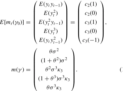
While the second moments of the data do not identifyγ = (θ, σ2)′, would the three nonzero third moments given by
achieve identification? The following lemma provides an answer to this question.
same dimension. Part (a) states that there always exist γ1, γ2∈Ŵ that are observationally equivalent in the sense
that they generate the same moments. For example, γ1=
(θ, σ2, κ
3)′ and γ2=(1/θ, θ2σ2, θ κ3)′ both imply the same
(E(ytyt−1), E(yt2), E(yt2yt−1))′. Part (b) of Lemma 1 follows
from the fact that the determinant of the derivative matrix is zero at|θ| =1. As a result, a single third moment cannot be guaran-teed to identify bothκ3and the parameters of the MA(1) model
θandσ2. Global and local identification ofθat
|θ| =1 requires use of information in the remaining two third-order moments. In particular, the derivative matrix ofg(γ)=(g′
2, g3′)′with
re-spect toγ =(θ, σ2, κ3)′is of full column rank everywhere in
Ŵincluding|θ| =1. However, sinceg(·) is of dimension five, this together with Lemma 1 implies that γ can only be over-identified if κ3=0. The next subsection describes a general
procedure, based on higher order cumulants, for identifying the parameters of MA(q) and ARMA (p,q) models.
3.2 The MA(q) Model
The insight from the MA(1) analysis that the parameters of the model cannot be exactly identified but can be over-identified with an appropriate choice of higher order moments extends to MA(q) models. But for MA(q) models, the moments of the process are nonlinear functions of the model parameters and verifying global and local identification is more challenging. Our analysis is built on results from the statistical engineering literature.
Letcℓ(τ1, τ2, . . . , τℓ−1) be theℓth (ℓ≥2)-order cumulant of
a zero-mean stationary and ergodic processyt. The second- and third-order cumulants ofyt are given by
c2(τ1)=E(ytyt+τ1),
Higher order cumulants are useful for identification of pos-sibly noninvertible models because the Fourier transform of cℓ(τ1, τ2, . . . , τℓ−1) is theℓth-order polyspectrum Recovery of phase information necessarily requires thatet has non-Gaussian features. In other words, ηℓ must exist and is nonzero for someℓ≥3 for recovery of the phase function; see Lii and Rosenblatt (1982, Lemma 1), Giannakis and Swami (1992), Giannakis and Mendel (1989), Mendel (1991), Tugnait (1986), and Ramsey and Montenegro (1992).
To establish that the MA(q) parameters are identifiable from cumulants of a particular orderℓ, the typical starting point is to generate identities that link the second and higher order cumu-lants to the parameters of the model. Different identities exist for different choice ofτ1, τ2, . . . , τℓ−1. Mendel (1991) provided
a survey of the methods used in the engineering literature. One of the simplest and earliest ideas is to consider the diagonal slice of the third-order cumulants, which implies the following relation between the population cumulants and theq+1 vector of parametersγ =(θ1, . . . , θq, κ3σ)′:
The system of Equation (7) can be expressed as
Aβ(γ)=b. (8) The reason why (8) is useful for identification is thatAβ(γ)= b is an over-identified system of 3q+1 equations in 2q+1 unknownsβ(γ). The parametersγ are identifiable ifβ(γ) can be solved from (8). Given that the derivative matrix ofβ(γ) with respect toγhas rankq+1, the identification problem reduces to the verification of the column rank of the matrixA(given in the Appendix).
Lemma 2. Consider the MA(q) process yt=et+
θ1et−1+ · · · +θqet−q, where et=σ εt, εt ∼iid(0,1) with
κ3=E(εt3)=0 and E|εt|3<∞. Let cℓ(τ) denote the diag-onal slice of theℓth-order cumulant ofyt. Ifc2(q) andc3(q) are
nonzero, then the matrixAhas full column rank 2q+1. A proof is given in the Appendix. Full rank of the ma-trix A enables identification of β(γ) and subsequently of γ. This requires that the qth autocorrelation c2(q) is nonzero,
and also that c3(q)=0. In view of the definition ofc3(q) in
(5), it is clear that skewness in et is necessary for identifica-tion of γ. A similar idea can be used to analyze identifica-tion using fourth-order cumulants, defined as c4(τ1, τ2, τ3)=
E(ytyt+τ1yt+τ2yt+τ3) −c2(τ1)c2(τ2−τ3)−c2(τ2)c2(τ3−τ1)−
c2(τ3)c2(τ1−τ2). For example, the diagonal slice of the
fourth-order cumulants yields a system of equations given by
q
Nondiagonal slices of the fourth-order cumulants were consid-ered by Friedlander and Porat (1990) and Na et al. (1995).
Giannakis and Mendel (1989, p. 364) made use of the struc-ture of theAmatrix to recursively compute the parameters in β(γ) and henceγ. This algorithm treatsκ3σ θ12, . . . , κ3σ θq2 as free parameters when, in fact, they are not. Although the method is not efficient or practical for estimation, the approach is one of the first to suggest the possibility of identification of MA models using cumulants. Tugnait (1995) subsequently obtained closed-form expressions for the MA parameters usingc3(τ, τ+q) and
autocovariances. Friedlander and Porat (1990) proposed an op-timal minimum distance estimation of the system (8) although this method still cannot separately identify the parametersκ3
(or κ4) and σ2. As we will see below, this approach is a
re-stricted version of our proposed GMM method.
3.3 ARMA(p,q) Model
The previous two subsections have focused on MA(q) models because thepparameters in the autoregressive polynomialα(L) can be easily identified. Consider the ARMA(p, q) model
yt =α1yt−1+ · · · +αpyt−p =et+θ1et−1+ · · · +θqet−q,
Thep×pToeplitz matrix on the right-hand side is a submatrix of autocovariances and hence full rank. Thus,αis identifiable. By considering the spectrum atpfrequencies, identities can also be derived in the frequency domain. Ifet were non-Gaussian, the AR coefficients of an ARMA process can still be uniquely determined from the equationspi=0
p
j=0αiαjcℓ(τ1−i, τ2−
j, τ3, . . . , τℓ−1)=0 forℓ≥3 and |τ1−τ2|> q. The idea of
using cumulants to identify the autoregressive parameters seems to date back to Akaike (1966), see Mendel (1991, p. 281) and Theorem 2 of Giannakis and Swami (1992).
The question then arises as to whether (α1, . . . , αp,
θ1, . . . , θq)′ can be jointly identified from the third-order cu-mulants alone. TheAβ(γ)=bframework presented above re-quires thatqis finite and hence does not work for ARMA(p, q) models. Assuming that the ARMA model has no common fac-tors (hence, it is irreducible), the following lemma, adapted from Tugnait (1995), provides sufficient conditions for identifiability of the parameters of ARMA(p, q) models.
Lemma 3. Assume that the ARMA(p, q) process (1−α1L−
· · · −αpLp)yt =(1+θ1L+ · · · +θqLq)et is irreducible and satisfies pi=0αizi =0 for |z| =1, where et=σ εt, εt ∼ iid(0,1) withκ3=E(ε3t)=0 andE|εt|3<∞. Letcℓ(τ) denote the diagonal slice of theℓth-order cumulant of the MA(p+q) process (1−α1L− · · · −αpLp)(1+θ1L+ · · · +θqLq)etand assume that c2(p+q) andc3(p+q) are nonzero. Then, the
parameter vector (α1, . . . , αp, θ1, . . . , θq)′of the ARMA(p,q) process is identifiable from the second and third cumulants of the MA(p+q) process.
The thrust of the argument, elaborated in the Appendix, is that observational equivalence of the two ARMA(p, q) process amounts to equivalence of two appropriately defined MA(p+q) processes, say, z, parameterized byp+q vectors1 and2,
respectively. But from Tugnait (1995), two MA(p + q) pro-cesses are equivalent ifc3z(τ1, p+q|1)=c3z(τ1, p+q|2)
for 0≤τ1≤p+q. We can now exploit results from the
previ-ous subsection. Tugnait (1995) used information in the nondi-agonal slices to isolate the smallest number of third and higher order cumulants that are sufficient for identification of ARMA parameters.
The representationAβ(γ)=bprovides a transparent way to see how higher order cumulants can be used to recover the pa-rameters of the model without imposing invertibility. However, this approach may use more cumulants than is necessary. To see why, (5) implies that for an MA(q) process,c3(q, k)=κ3σ3θqθk andc3(q,0)=κ3σ3θq. It immediately follows thatθk= cc3(q,k)
3(q,0).
This so-calledC(q, k) formula suggests that onlyq+1 third-order cumulantsc3(q, τ) for 0≤τ ≤qare necessary and
suffi-cient for identification ofθ1, . . . , θq ifκ3=0, which is smaller
than the number of equations in theAβ(γ)=bsystem. The key point in this section to highlight is that once non-Gaussian features are allowed, identification of noninvertible models is possible from the higher order cumulants of the data. In practice, we would want to use the covariance structure along with identities based on the third- and fourth-order cumulants. Using information in the third or fourth cumulants alone would be inefficient, even though identification is possible. This is because the covariance structure would have been sufficient for identification if invertibility was imposed, and the fourth-order
cumulants can be useful when the error distribution is (near-) symmetric. The identities considered shed light on which order cumulants are required for identification. For example, in the MA(1) case, theAβ(γ)=bsystem
be needed to identify the MA(1) parameters. This is used to guide estimation, which is the subject of the next section.
4. GMM ESTIMATION
The results in Section3suggest to estimate the parameters of ARMA(p, q) models by matching second and higher order cu-mulants. Friedlander and Porat (1990, p. 30) proposed a two-step procedure for estimating ARMA(p,q) models where the AR pa-rameters are obtained first from the autocovariances (spectrum) of the process and the MA parameters are then estimated from the filtered process using information in the higher order cu-mulants (a similar estimation strategy has been proposed by an anonymous referee). Our proposed estimation strategy is similar in spirit but it estimates all of the unknown parameters in one step.
Let gt(γ) be conditions characterizing the model parame-terized by γ and such that at the true value γ0, E[gt(γ0)]= denote a consistent estimate of the positive definite matrix =limT→∞var(
sufficient forγ0to be a unique solution to the system of nonlinear
equations characterized by G(γ)′−1g(γ)
=0.The full rank condition in the neighborhood of γ0 is also necessary for the
estimator to be asymptotically normal. Under the assumptions given by Newey and McFadden (1994),
√
Consistent estimation of possibly noninvertible ARMA(p, q) models depends on the choicegt(γ). We consider three possi-bilities beginning with a classical GMM estimator.
For the MA(1) model, letγ =(θ, σ2, κ
3)′be the parameters
to be estimated and define
g(γ)=m(γ0)−m(γ),
Note that the equations in (11) are particular linear combinations of the moment conditions in (14). The conditions in Lemma 2 thatc2(1)=0 andc3(1)=0 correspond to the conditionsθ=0
andκ3 =0 in Lemma 1.
Proposition 1. Consider the MA(1) model. Suppose that in addition to the assumptions in Lemma 1, we have that E|et|6<∞ and γ0 is in the interior of the compact param-Then,γis√T consistent with asymptotic distribution given by (13).
The derivative matrixG(γ)= ∂g∂γ(γ′)is of full column rank
ev-erywhere inŴ(even at|θ| =1). As a result, this GMM estimator is root-T consistent and asymptotically normal.
4.1 Finite-Sample Properties of the GMM Estimator
To illustrate the finite-sample properties of the GMM esti-mator, data withT =500 observations are generated from an MA(1) modelyt =et+θ et−1andet =σ εt, whereεtis iid(0,1) and follows a GLD, which will be further discussed in Section 5.1. For now, it suffices to note that GLD distributions can be characterized by a skewness parameterκ3and a kurtosis
parame-terκ4.The true values of the parameters areθ=0.5,0.7,1,1.5,
and 2,σ =1,κ3 =0,0.35,0.6, and 0.85, andκ4=3. The
re-sults are invariant to the choice of σ. Lack of identification of γ arises when κ3=0 and weak to intermediate
identifi-cation occurs when κ3=0.35 and 0.6. Unreported numerical
results revealed that the estimator based on the moment condi-tions (14) possesses substantially better finite-sample properties than the estimator based on (11). We only consider the finite-sample properties of the estimator for the MA(1) model when the orthogonality conditions are both necessary and sufficient for identification.
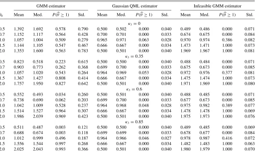
Table 1 presents the mean, the median, and the standard deviation of three estimators of θ over 1000 Monte Carlo replications. The first is the GMM estimator ofγ =(θ, σ2, κ3)′,
which uses (14) as moment conditions. The second is the infeasible GMM estimator based on (14) but assumes σ2 is known and estimates only (θ, κ3)′. As discussed earlier,
fixing σ2 solves the identification problem in the MA(1) model, and by not imposing invertibility,|θ| =1 is not on the boundary of the parameter space forγ. We will demonstrate
Table 1. GMM and Gaussian QML estimates ofθfrom MA(1) model with possibly asymmetric errors
GMM estimator Gaussian QML estimator Infeasible GMM estimator
θ0 Mean Med. P(θ≥1) Std. Mean Med. P(θ≥1) Std. Mean Med. P(θ≥1) Std.
κ3=0
0.5 1.392 1.692 0.578 0.790 0.500 0.502 0.000 0.040 0.489 0.486 0.000 0.071
0.7 1.152 1.117 0.564 0.428 0.700 0.701 0.000 0.033 0.674 0.675 0.000 0.084
1.0 1.057 1.004 0.509 0.279 0.965 0.971 0.063 0.028 0.970 0.974 0.386 0.082
1.5 1.144 1.105 0.547 0.467 0.666 0.667 0.000 0.034 1.473 1.471 1.000 0.073
2.0 1.353 1.600 0.563 0.783 0.500 0.501 0.000 0.040 1.969 1.967 1.000 0.081
κ3=0.35
0.5 0.823 0.518 0.223 0.615 0.500 0.500 0.000 0.040 0.488 0.484 0.000 0.071
0.7 0.903 0.773 0.262 0.368 0.699 0.700 0.000 0.033 0.675 0.673 0.000 0.085
1.0 1.057 1.020 0.543 0.264 0.964 0.969 0.053 0.028 0.972 0.976 0.377 0.081
1.5 1.367 1.427 0.808 0.414 0.666 0.667 0.000 0.034 1.475 1.474 1.000 0.073
2.0 1.757 1.950 0.827 0.642 0.500 0.501 0.000 0.040 1.971 1.969 1.000 0.080
κ3=0.6
0.5 0.552 0.493 0.034 0.260 0.500 0.501 0.000 0.040 0.488 0.485 0.000 0.071
0.7 0.738 0.690 0.062 0.203 0.699 0.700 0.000 0.033 0.677 0.673 0.000 0.085
1.0 1.042 1.009 0.528 0.237 0.964 0.968 0.048 0.028 0.975 0.982 0.389 0.077
1.5 1.514 1.527 0.964 0.307 0.666 0.667 0.000 0.034 1.478 1.478 1.000 0.069
2.0 1.986 2.039 0.969 0.423 0.500 0.501 0.000 0.040 1.975 1.973 1.000 0.076
κ3=0.85
0.5 0.511 0.487 0.003 0.121 0.500 0.500 0.000 0.040 0.489 0.485 0.000 0.069
0.7 0.688 0.674 0.003 0.118 0.699 0.699 0.000 0.033 0.678 0.677 0.000 0.084
1.0 1.012 0.999 0.496 0.187 0.964 0.966 0.046 0.027 0.978 0.987 0.416 0.072
1.5 1.556 1.544 0.997 0.268 0.666 0.667 0.000 0.034 1.482 1.483 1.000 0.063
2.0 2.025 2.043 0.993 0.366 0.500 0.501 0.000 0.040 1.980 1.979 1.000 0.070
NOTES: The table reports the mean, median (med.), probability thatθ≥1, and standard deviation (std.) of the GMM, Gaussian quasi-maximum likelihood (QML), and infeasible GMM estimates ofθfrom the MA(1) modelyt=et+θ et−1, whereet=σ εt andεt∼iid(0,1) are generated from a generalized lambda distribution (GLD) with a skewness
parameterκ3and no excess kurtosis. The sample size isT=500, the number of Monte Carlo replications is 1000 andσ=1. The GMM estimator is based on the moment conditions
(E(ytyt−1)−θ σ2, E(yt2)−(1+θ2)σ2, E(yt2yt−1)−θ2σ3κ3, E(yt3)−(1+θ3)σ3κ3, E(ytyt2−1)−θ σ3κ3)′. The infeasible GMM estimator is based on the same set of moment conditions
but withσ=1 assumed known. Both GMM estimators use the optimal weighting matrix based on the Newey–West HAC estimator with automatic lag selection.
that our proposed GMM estimator has properties similar to this infeasible estimator. The third is the Gaussian quasi-ML estimator of (θ, σ2)′with invertibility imposed, which is used to evaluate the efficiency losses of the GMM estimator for values ofθin the invertible region (θ=0.5 and 0.7).
The results inTable 1 suggest that regardless of the degree of non-Gaussianity, the infeasible estimator produces estimates ofθ that are very precise and essentially unbiased. Hence, fix-ingσ solves both identification problems without the need of non-Gaussianity although a prior knowledge ofσis rarely avail-able in practice. By construction, the Gaussian QML estimator imposes invertibility and works well when the true MA param-eter is in the invertible region but cannot identify the paramparam-eter values in the noninvertible region. While forκ3=0.35 the
iden-tification is weak and the estimates ofθ are somewhat biased, for higher values of the skewness parameter the GMM estimates ofθare practically unbiased.
Table 1also presents the empirical probability that the partic-ular estimator ofθis greater than or equal to one, which provides information on how often the identification of the true parameter fails. The Gaussian QML estimator is characterized by a pile-up probability at unity (which can be inferred fromP(θ≥1) whenθ0=1) as argued before. Even whenκ3=0.35, the GMM
estimator correctly identifies if the true value ofθ is in the in-vertible or the noninin-vertible region with high probability. This probability increases whenκ3=0.85.
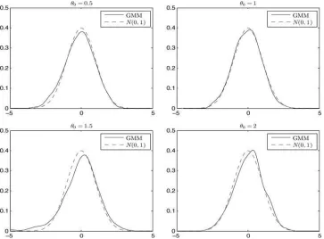
Finally, to assess the accuracy of the asymptotic normal-ity approximation in Proposition 1,Figure 1 plots the density
functions of the standardized GMM estimator (t-statistic) ofθ for the MA(1) model with GLD errors and a skewness parameter of 0.85 (strong identification). The sample size isT =3000 and θ =0.5,1,1.5, and 2. Overall, the densities of the standardized GMM estimator appear to be very close to the standard normal density for all values ofθ. The coverage probabilities of the 90% confidence intervals for θ=0.5,0.7,1,1.5, and 2 are 91.8%, 90.5%, 92.6%, 89.5%, and 92.9%, respectively.
5. SIMULATION-BASED ESTIMATION
A caveat of the GMM estimator is that it relies on pre-cise estimation of the higher order unconditional moments, but finite-sample biases can be nontrivial even for samples of mod-erate size. This can be problematic for GMM estimation of ARMA(p, q) models since a large number of higher order terms needs to be estimated. To remedy these problems, we consider the possibility of using simulation to correct for finite-sample biases (see Gourieroux, Renault, and Touzi1999; Phillips2012). Two estimators are considered. The first is a simulation analog of the GMM estimator, and the second is a simulated minimum distance estimator that uses auxiliary regressions to efficiently incorporate information in the higher order cumulants into a parameter vector of lower dimension. Both estimators can ac-commodate additional dynamics, kurtosis, and other features of the errors.
Simulation estimation of the MA(1) model was considered in Gourieroux, Monfort, and Renault (1993), Michaelides and Ng
Figure 1. Density functions of the standardized GMM estimator (t-statistic) ofθbased on data (T =3000) generated from an MA(1) model yt =et+θ et−1withθ=0.5,1,1.5,2, andet ∼iid(0,1). The errors are drawn from a generalized lambda distribution with zero excess kurtosis
and a skewness parameter equal to 0.85. For the sake of comparison, the figure also plots the standard normal (N(0,1)) density.
(2000), Ghysels, Khalaf, and Vodounou (2003), and Czellar and Zivot (2008), among others, but only for the invertible case. All of these studies use an autoregression as the auxiliary model. For θ=0.5 and assuming thatσ2is known, Gourieroux, Monfort,
and Renault (1993) found that the simulation-based estimator compares favorably to the exact ML estimator in terms of bias and root mean squared error. Michaelides and Ng (2000) and Ghysels, Khalaf, and Vodounou (2003) also evaluated the prop-erties of simulation-based estimators withσ2assumed known. Czellar and Zivot (2008) reported that the simulation-based es-timator is relatively less biased but exhibits some instability and the tests based on it suffer from size distortions whenθ0is close
to unity (see also Tauchen1998for the behavior of simulation estimators near the boundary of the parameter space).
5.1 The GLD Error Simulator
The key to identification is errors with non-Gaussian features. Thus, in order for any simulation estimator to identify the pa-rameters without imposing invertibility, we need to be able to simulate non-Gaussian errorsεtin a flexible fashion so thatyt has the desired distributional properties.
There is evidently a large class of distributions with third and fourth moments consistent with a non-Gaussian process that one can specify. Assuming a particular parametric error distribution could compromise the robustness of the estimates. We simulate errors from the GLD(λ1, λ2, λ3, λ4) considered
in Ramberg and Schmeiser (1975). This distribution has two appealing features. First, it can accommodate a wide range of values for the skewness and excess kurtosis parameters and it includes as special cases normal, log-normal, exponential, t,
beta, gamma, and Weibull distributions. The second advantage is that it is easy to simulate from. The percentile function is given by
(u)−1 =λ1+[Uλ3+(1−U)λ4]/λ2, (15)
where U is a uniform random variable on [0,1], λ1 is a
lo-cation parameter, λ2 is a scale parameter, and λ3 andλ4 are
shape parameters. To simulateεt, aU is drawn from the uni-form distribution and (15) is evaluated for given values of (λ1, λ2, λ3, λ4). Furthermore, the shape parameters (λ3, λ4) and
the location/scale parameters (λ1, λ2) can be sequentially
eval-uated. Sinceεthas mean zero and variance one, the parameters (λ1, λ2) are determined by (λ3, λ4) so thatεtis effectively char-acterized byλ3andλ4. As shown in Ramberg and Schmeiser
(1975), the shape parameters (λ3, λ4) are explicitly related to
the coefficients of skewness and kurtosis (κ3 andκ4) ofεt (see the Appendix). A consequence of having to use the GLD to simulate errors is that the parametersλ3 andλ4 of the GLD
distribution must now be estimated along with the parameters ofyt, even though these are not parameters of interest per se. In practice, these GLD parameters are identified from the higher order moments of the residuals from an auxiliary regression.
5.2 The SMM Estimator
Define the augmented parameter vector of the MA(1) model asγ+=(θ, σ2, λ
3, λ4)′.Our SMM estimator is based on
g(γ+)=T1 T
t=1
mt(γ0+)−
1 T S
T S
t=1
mSt(γ+), (16)
where mt(γ0+) is evaluated on the observed data y=
(y1, . . . , yT)′ andmSt(γ+) is evaluated on the datay S
(γ+)= (y1S, . . . , yTS, . . . , yT SS )′ of lengthT S (S≥1), simulated for a candidate value ofγ+. Essentially, the quantitym(γ+) which is chosen to summarize the dependence of the model on the parametersγ+is approximated by Monte Carlo methods.
It remains to definemt(γ0+). In contrast to GMM estimation,
we now need moments of the innovation errors to identifyλ3
andλ4. The latent errors are approximated by the standardized
residuals from estimation of an AR(p) model
yt =π0+π1yt−1+ · · · +πpyt−p+σ ǫt. For the MA(1) model, the moment conditions given by
mt(γ0+)=
ytyt−1 y2t y
2
tyt−1 y3t ytyt2−1 y 3
tyt−1 ytyt3−1
yt2yt2−1 yt4 ǫˆt3 ǫˆt4′ (17) reflect information in the second-, third-, and fourth-order cu-mulants of the processyt, as well as skewness and kurtosis of the errors.
To establish the consistency and asymptotic normality of the SMM estimatorγ+, we need some additional notation and reg-ularity conditions. Let Fe denote the true distribution of the structural model errors and∗be the class of GLDs.
Proposition 2. Consider the MA(1) model and let G(γ+)=∂g(γ+)/∂γ+′, G(γ+)=∂g(γ+)/∂γ+′, and = limT→∞var(
√
T g(γ+)). In addition to the assumptions in Lemma 1, assume thatFe∈∗,E|et|8<∞, supγ∈Ŵ|G(γ+)− G(γ+)|−→p 0, γ+
0 is in the interior of the compact parameter
spaceŴ+, and√T g(γ0+)−→d N(0, ). Then, √
T(γ+−γ+
0 )
d −→N
0,
1+ 1
S
G(γ0+)′−1G(γ0+)−1
≡N0,Avar(γ+).
Consistency follows from identifiability ofγ and the higher order cumulants play a crucial role. In our procedure,κ3andκ4
are defined in terms ofλ3andλ4. Thus,λ3andλ4are crucial for
identification ofθandσ2even though they are not parameters of direct interest.
A key feature of Proposition 2 is that it holds whenθis less than, equal to, or greater than one. In a Gaussian likelihood setting when invertibility is assumed for the purpose of iden-tification, there is a boundary for the support ofθ at the unit circle. Thus, the likelihood-based estimation has nonstandard properties when the true value ofθ is on or near the boundary of one. In our setup, this boundary constraint is lifted because identification is achieved through higher moments instead of imposing invertibility. As a consequence, the SMM estimator
γ+has classical properties provided thatκ3andκ4enable iden-tification.
Consistent estimation of the asymptotic variance ofγ+ can proceed by substituting a consistent estimator ofand evalu-ating the JacobianG(γ+) numerically. The computed standard errors can then be used for testing hypotheses and constructing confidence intervals. Inference on the MA parameter of interest, θ, can also be conducted by constructing confidence intervals
based on inversion of the distance metric test without an ex-plicit computation of the variance matrix Avar(γ+). It should be stressed that despite the choice of a flexible functional distribu-tional form for the error simulator, our structural model is still correctly specified. This is in contrast with the semiparametric indirect inference estimator of Dridi, Guay, and Renault (2007). They considered partially misspecified structural models and thus required an adjustment in the asymptotic variance of the estimator.
5.3 The SMD Estimator
Higher order MA(q) models and general ARMA(p, q) mod-els can in principle be estimated by GMM or SMM. But as mentioned earlier, the number of orthogonality conditions increases with p and q. Instead of selecting additional mo-ment conditions, we combine the information in the cumu-lants into the auxiliary parameters that are informative about the parameters of interest. Letψ(γ0+)=arg minψQT(ψ;y) and
ψS(γ+)=arg min
ψQT(ψ;yS(γ+)) be the auxiliary parameters
estimated from actual and simulated data,QT(·) denotes the ob-jective function of the auxiliary model, and is a consistent estimate of the asymptotic variance ofψ. Our simulated mini-mum distance (SMD) based on
g(γ+)=ψ(γ0+)−ψS(γ+) (18) shares the same asymptotic properties as the SMM estimator in Proposition 2. The SMD estimator is in the spirit of the indi-rect inference estimation of Gourieroux, Monfort, and Renault (1993) and Gallant and Tauchen (1996). Their estimators require that the auxiliary model is easy to estimate and that the mapping from the auxiliary parameters to the parameters of interest is well defined. We use such a mapping to collect information in the unconditional cumulants into a lower dimensional vector of auxiliary parameters to circumvent direct use of a large number of unconditional cumulants.
We consider least-square (LS) estimation of the auxiliary regressions
yt =π0+π1yt−1+ · · · +πpyt−p+σ ǫt, (19a)
yt2=c0+c1,1yt−1+ · · · +c1,ryt−r+c2,1y2t−1
+ · · · +c2,ryt2−r+vt (19b) with an appropriate choice ofpandr. Equation (19a) has been used in the literature for simulation estimation of MA(1) mod-els when invertibility is imposed, and often withσ2 assumed
known. We complement (19a) with the regression defined in (19b). The parameters of this regression parsimoniously sum-marize information in the higher moments of the data. Compared to the SMM in which the auxiliary parameters are unconditional moments, the auxiliary parametersψare based on conditional moments. Equation (19b) also provides a simple check for the prerequisite for identification. If the c coefficients are jointly zero, identification would be in jeopardy.
Letκ3 andκ4 denote the sample third and fourth moments
of the ordinary LS (OLS) residuals in (19a). The auxiliary
Table 2. SMM and SMD estimates ofθfrom MA(1) model with asymmetric errors
SMM SMD
Mean Med. P(θ≥1) Std. Mean Med. P(θ≥1) Std.
GLD,σt =σ
θ0=0.5 0.488 0.484 0.001 0.054 0.503 0.503 0.000 0.043
θ0=0.7 0.693 0.688 0.000 0.083 0.705 0.703 0.002 0.053
θ0=1.0 0.949 0.988 0.421 0.137 0.973 0.982 0.406 0.089
θ0=1.5 1.563 1.520 0.962 0.280 1.482 1.493 0.980 0.104
θ0=2.0 1.903 1.959 0.940 0.337 1.996 1.995 0.988 0.180
GLD+ARCH
θ0=0.5 0.437 0.426 0.013 0.064 0.549 0.479 0.062 0.055
θ0=0.7 0.648 0.636 0.006 0.099 0.748 0.687 0.143 0.059
θ0=1.0 0.929 0.959 0.318 0.160 1.068 1.087 0.790 0.117
θ0=1.5 1.573 1.561 0.940 0.274 1.483 1.486 0.983 0.113
θ0=2.0 1.861 1.956 0.883 0.374 1.926 1.924 0.978 0.240
NOTES: The table reports the mean, median (med.), probability thatθ≥1, and standard deviation (std.) of the SMM estimates ofθfrom the MA(1) modelyt=et+θ et−1, where
et=σtεt, εt∼iid(0,1) are generated from a generalized lambda distribution (GLD) with a skewness parameterκ3=0.85 (and no excess kurtosis) andσt=σ=1 orσt2=0.7+0.3e2t−1.
The sample size isT=500 and the number of Monte Carlo replications is 1000. The SMM estimator is based on the moment conditionsmSMM,t, defined in (17), and the SMD estimator
is based on the auxiliary parameter vectorψSMD, defined in (19c). The SMM and SMD estimators use the optimal weighting matrix based on the Newey–West HAC estimator.
parameter vector based on the data is
ψ(γ0+)=π0,π1, . . . ,πp,c0,c1,1, . . . ,c1,r,c2,1,
. . . ,c2,r,κ3,κ4
′.
(19c)
The parameter vector ψS(γ+) is analogously defined, except that the auxiliary regressions are estimated with data simulated for a candidate value ofγ.
5.4 Finite-Sample Properties of the Simulation-Based Estimators
To implement the SMM and SMD estimators, we simulateT S errors from the generalized lambda error distribution. Larger values ofS (the number of simulated sample paths of length T) tend to smooth the objective functions, which improves the identification of the MA parameter. As a result, we setS=20
Figure 2. Logarithm of the objective function of simulation-based estimator ofθandσbased on data (T =1000) generated from an MA(1) modelyt=et +θ et−1withθ=0.7 andet ∼iid(0,1). The errors are drawn from a generalized lambda distribution with zero excess kurtosis
and a skewness parameter equal to 0, 0.35, 0.6, and 0.85.
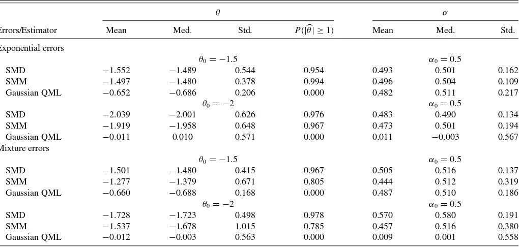
Table 3. SMD, SMM, and Gaussian QML estimates ofθandαfrom an ARMA(1, 1) model with exponential/mixture of normals errors
θ α
Errors/Estimator Mean Med. Std. P(|θ| ≥1) Mean Med. Std.
Exponential errors
θ0= −1.5 α0=0.5
SMD −1.552 −1.489 0.544 0.954 0.493 0.501 0.162
SMM −1.497 −1.480 0.378 0.994 0.496 0.504 0.109
Gaussian QML −0.652 −0.686 0.206 0.000 0.482 0.511 0.217
θ0= −2 α0=0.5
SMD −2.039 −2.001 0.626 0.976 0.483 0.490 0.134
SMM −1.919 −1.958 0.648 0.967 0.473 0.501 0.194
Gaussian QML −0.011 0.010 0.571 0.000 0.011 −0.003 0.567
Mixture errors
θ0= −1.5 α0=0.5
SMD −1.501 −1.480 0.415 0.967 0.505 0.516 0.137
SMM −1.277 −1.379 0.671 0.805 0.444 0.512 0.319
Gaussian QML −0.660 −0.688 0.168 0.000 0.487 0.510 0.186
θ0= −2 α0=0.5
SMD −1.728 −1.723 0.498 0.978 0.570 0.580 0.191
SMM −1.537 −1.678 1.015 0.785 0.457 0.516 0.380
Gaussian QML −0.012 −0.003 0.563 0.000 0.009 0.001 0.558
NOTES: The table reports the mean, median (med.), standard deviation (std.), and the probability thatP(|θ| ≥1) of the SMD, SMM, and Gaussian QML estimates ofθandαfrom the ARMA(1, 1) model (1−αL)yt=(1+θ L)et, whereet=σ εtandεtis an exponential random variable with a scale parameter equal to one (exponential errors) or a mixture of normals
random variable with mixture probabilities 0.1 and 0.9, means−0.9 and 0.1, and standard deviations 2 and 0.752773, respectively (mixture errors). The exponential errors are recentered and rescaled to have mean zero and variance one. The sample size isT=500 and the number of Monte Carlo replications is 1000.
althoughS >20 seems to offer even further improvement, es-pecially for smallT ,but at the cost of increased computational time. The SMM and SMD estimators both usep=4. SMD additionally assumesr =1 in the auxiliary model (19b).
As is true of all nonlinear estimation problems, the numerical optimization problem must take into account the possibility of local minima, which arises when the invertibility condition is not imposed. Thus, the estimation always considers two sets of initial values. Specifically, we draw two starting values for θ—one from a uniform distribution on (0,1) and one from a uniform distribution on (1,2)—with the starting value forσ set equal toσ2
y/(1+θ2) for each of the starting values forθ. The starting values for the shape parameters of the GLDλ3andλ4
are set equal to those of the standard normal distribution (with κ3=0 andκ4=3). In this respect, the starting values ofθ,σ,
λ3, andλ4contain little prior knowledge of the true parameters.
MA(1). In the first experiment, data are generated from
yt =et+θ et−1, et =σtεt,
where εt ∼iid(0,1) is drawn from a GLD with zero excess kurtosis and a skewness parameter 0.85 with (i)σt =σ =1 or (ii)σt =0.7+0.3e2t−1 (ARCH errors). The sample size is
T =500, the number of Monte Carlo replications is 1000 and θ takes the values of 0.5, 0.7, 1, 1.5, and 2. Note that the structural model used for SMM and SMD does not impose the ARCH structure of the errors, that is, the error distribution is misspecified. This case is useful for evaluating the robustness properties of the proposed SMM and SMD estimators.
Table 2 reports the mean and median estimates of θ, the standard deviation of the estimates for which identification is achieved and the probability that the estimator is equal to or greater than one. When the errors are iid drawn from the GLD
distribution, the SMM estimator ofθexhibits only a small bias for some values of θ (e.g., θ0=2). While there is a positive
probability that the SMM estimator will converge to 1/θ in-stead ofθ (especially whenθ is in the noninvertible region), this probability is fairly small and it disappears completely for largerT(not reported to conserve space). When the error distri-bution is misspecified (GLD errors with ARCH structure), the properties of the estimator deteriorate (the estimator exhibits a larger bias) but the invertible/noninvertible values ofθare still identified with high probability. However, the SMD estimator provides a substantial bias correction, efficiency gain, and iden-tification improvement. Interestingly, in terms of precision, the SMD estimator appears to be more efficient than the infeasible estimator inTable 1for values ofθin the invertible region. The SMD estimator continues to perform well even when the error simulator is misspecified.
Figure 2illustrates how identification depends on skewness by plotting the log of the objective function for the SMD estima-tor averaged over 1000 Monte Carlo replications of the MA(1) model withθ=0.7 andσ =1. The errors are generated from GLD with zero excess kurtosis and three values of the skewness parameter: 0, 0.35, 0.6, and 0.85. In evaluating the objective function, the values of the lambda parameters in the GLD are set equal to their true values. The first case (no skewness) cor-responds to lack of identification and there are two pronounced local minima atθand 1/θ.As the skewness of the error distri-bution increases, the second local optima at 1/θflattens out and it almost completely disappears when the error distribution is highly asymmetric.
ARMA(1, 1). In the second simulation experiment, data are generated according to
yt =αyt−1+et+θ et−1, (20)
where et is (i) a standard exponential random variable with a scale parameter equal to one, which is recentered and rescaled to have mean zero and variance 1 or (ii) a mixture of normals random variable with mixture probabilities 0.1 and 0.9, means −0.9 and 0.1, and standard deviations 2 and 0.752773, respec-tively. The second error distribution is included to assess the robustness properties of the simulation-based estimator to error distributions that are not members of the GLD family.
We consider two parameterizations that give rise to a causal process with a noninvertible MA component. The first param-eterization is α=0.5 and θ= −1.5. The second parameteri-zation, α=0.5 and θ= −2, produces an all-pass ARMA(1, 1) process, which is characterized byθ= −1/α. This all-pass process possesses some interesting properties (see Davis2010). First,ytis uncorrelated but is conditionally heteroscedastic. Sec-ond, if one imposes invertibility by lettingθ= −αand scale up the error variance by (1/α)2, the process is iid and the AR and
MA parameters are not separately identifiable. Imposing invert-ibility in such a case is not innocuous, and estimation of the parameters of this model is quite a challenging task.
Table 3presents the finite-sample properties of the SMD and SMM estimators for the ARMA(1, 1) model in (20) using the same auxiliary parameters and moment conditions for the esti-mation of MA(1). For comparison, we also include the Gaussian quasi-ML estimator. The SMD estimates ofθ appear unbiased for the exponential distribution and are somewhat downward biased for the mixture of normals errors. But, overall, the SMD estimator identifies correctly the AR and MA components with high probability. The performance of the SMM estimator is also satisfactory but it is dominated by the SMD estimator. The Gaussian QML estimator imposes invertibility and completely fails to identify the AR and MA parameters when α=0.5 and θ= −2. Even with a misspecified error distribution and a fairly parsimonious auxiliary model, the finite-sample proper-ties of our proposed simulation-based estimators remain quite attractive.
5.5 Empirical Application: 25 Fama-French Portfolio Returns
Noninvertibility can be consistent with economic theory. For example, supposeyt=Et
∞
s=0δ
sx
t+s is the present value of
xt=et+ωet−1. As shown by Hansen and Sargent (1991),
the solutionyt=(1+δω)et+ωet−1 =h(L)etimplies that the root of h(z) is−1+δω
ω , which can be on or inside the unit cir-cle even if |ω|<1. If there is no discounting and δ=1, yt has an MA unit root whenω= −0.5 andh(L) is noninvertible in the past whenever ω <−0.5. Note that even if an autore-gressive processes is causal, it is still possible for the roots of h(L)= δω(δδ)−−LωL (L) to be inside the unit disk.
Present value models are used to analyze variables with a for-ward looking component including stock and commodity prices. We estimate an MA(1) model for each of the 25 Fama-French portfolio returns using the Gaussian QML and the proposed SMM and SMD estimators. The data are monthly returns on the value-weighted 25 Fama-French size and book-to-market ranked portfolios from January 1952 until August 2013 (from Kenneth French’s website). The portfolios are the intersec-tions of five portfolios formed on size (market equity) and five
portfolios formed on the ratio of book equity to market equity. The size (book-to-market) breakpoints are the NYSE quintiles and are denoted by “small, 2, 3, 4, big” (“low, 2, 3, 4, high” ) in Table 4.
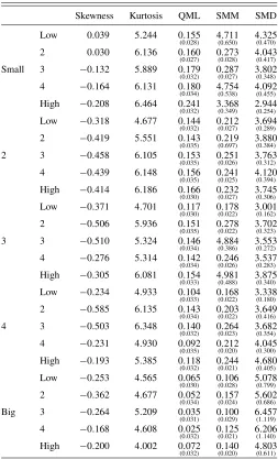
Table 4presents the sample skewness and kurtosis as well as the estimates and the corresponding standard errors (in paren-theses below the estimate) for each estimator and portfolio re-turn. All of the returns exhibit some form of non-Gaussianity, which is necessary for identifying possible noninvertible MA components. The Gaussian QML produces estimates of the MA coefficient that are small but statistically significant (with a few exceptions in the “big” size category). The SMM relaxes the invertibility constraint and delivers somewhat higher estimates of the MA parameter but most of these estimates still fall in the invertible region. By contrast, the SMD estimator suggests that all of the 25 Fama-French portfolio returns appear to be driven
Table 4. SMD, SMM, and Gaussian QML estimates of MA(1) model for stock portfolio returns
Skewness Kurtosis QML SMM SMD
Low 0.039 5.244 0.155
(0.028) 4(0..711650) 4(0..325470)
2 0.030 6.136 0.160
(0.027) 0(0..273028) 4(0..043417)
Small 3 −0.132 5.889 0.179
(0.032) 0(0..287027) 3(0..802348)
4 −0.164 6.131 0.180
(0.034) 4(0..754538) 4(0..092455)
High −0.208 6.464 0.241
(0.032) 3(0..368349) 2(0..944254)
Low −0.318 4.677 0.144
(0.032) 0(0..212027) 3(0..694289)
2 −0.419 5.551 0.143
(0.035) 0(0..219697) 3(0..880384)
2 3 −0.458 6.105 0.153
(0.035) 0(0..251026) 3(0..763312)
4 −0.439 6.148 0.156
(0.035) 0(0..241025) 4(0..120394)
High −0.414 6.186 0.166
(0.030) 0(0..232027) 3(0..745306)
Low −0.371 4.701 0.117
(0.030) 0(0..178022) 3(0..001162)
2 −0.506 5.936 0.151
(0.035) 0(0..278022) 3(0..702323)
3 3 −0.510 5.324 0.146
(0.034) 4(0..884386) 3(0..553272)
4 −0.276 5.314 0.142
(0.034) 0(0..246026) 3(0..537283)
High −0.305 6.081 0.154
(0.033) 4(0..981488) 3(0..875340)
Low −0.234 4.933 0.104
(0.033) 0(0..168022) 3(0..338180)
2 −0.585 6.135 0.143
(0.034) 0(0..203022) 3(0..649416)
4 3 −0.503 6.348 0.140
(0.032) 0(0..264023) 3(0..682354)
4 −0.231 4.930 0.092
(0.035) 0(0..212020) 4(0..045300)
High −0.193 5.385 0.118
(0.032) 0(0..244021) 4(0..680405)
Low −0.253 4.565 0.065
(0.030) 0(0..106028) 5(0..078799)
2 −0.362 4.677 0.052
(0.034) 0(0..157024) 5(0..602686)
Big 3 −0.264 5.209 0.035
(0.031) 0(0..100029) 6(1..457119)
4 −0.168 4.608 0.025
(0.032) 0(0..125021) 6(1..206140)
High −0.200 4.002 0.072
(0.032) 0(0..140020) 4(0..803611)
NOTES: The table reports the SMD, SMM, and Gaussian quasi-ML estimates and standard errors (in parentheses below the estimates) for the MA(1) modelyt=et+θ et−1, where
et∼iid(0, σ2) andytis one of the 25 Fama-French portfolio returns. The first two columns
report the sample skewness and kurtosis ofyt. The standard errors for SMM and SMD are
constructed using the asymptotic approximation in Proposition 2.
by a noninvertible MA component. The results are consistent with the finding through simulations that the SMD is more capa-ble of estimatingθ in the correct invertibility space. The SMD estimates are fairly stable across the different portfolio returns with a slight increase in their magnitude and standard errors for the “big” size portfolios. Also, a higher precision of the MA estimates is typically associated with returns that are character-ized by larger departures from Gaussianity. Overall, our SMD method provides evidence in support of noninvertibility in stock returns.
6. CONCLUSIONS
This article proposes classical and simulation-based GMM estimation of possibly noninvertible MA models with non-Gaussian errors. The identification of the structural parameters is achieved by exploiting the non-Gaussianity of the process through third-order cumulants. This type of identification also removes the boundary problem at the unit circle, which gives rise to the pile-up probability and nonstandard asymptotics of the Gaussian maximum likelihood estimator. As a conse-quence, the proposed GMM estimators are root-T consistent and asymptotically normal over the whole parameter range, pro-vided that the non-Gaussianity in the data is sufficiently large to ensure identification.
Other research questions arise once the assumption of invert-ibility is relaxed. A potential problem with the GMM estimator is that the number of orthogonality conditions can be quite large. This is especially problematic for ARMA(p, q) models. Ideally, the orthogonality conditions should be selected or weighted in an optimal fashion. More generally, how to determine the lag length of the heteroskedasticity and autocorrelation consistent (HAC) estimator without imposing invertibility remains a topic for future research.
APPENDIX: PROOFS
Proof of Lemma 1. The result in part (a) follows im-mediately by noticing that g(γ1) and g(γ2), where g= system of overdetermined equations but did not establish uniqueness of the solution. The argument for identification from third- and fourth-order cumulants (i.e., Equation (7)) and fourth-order cumulants (i.e., Equation (9)) are similar. We begin with (7).
Identification of MA(q) Models Using Third-Order Cumulants.The system of equations can be expressed asAβ(γ)=b, where rank of the submatrix consisting of B and D, and the rank of the submatrix consisting of C and E. The rank of the first subblock is determined by the rank of theq×q square matrixD, which isqif
respectively. Therefore,Ahas a full column rank of 2q+1 and the parameter vector β(γ) can be obtained as a unique solution to the system of Equation (8). Since the derivative matrix ofβ(γ) given by
is of full column rank, the parameter vector of interest γ=
(θ1, . . . , θq, κ3σ)′is identifiable.
Identification of MA(q) Models Using Fourth-Order Cumulants.The MA(q) model implies the following relation between the diagonal slices
of the fourth-order cumulants and theq+1 vector of parametersγ=
Then, the system of Equation (A.1) can be expressed as
Aβ(γ)=b
and the identification ofβ(γ) andγfollows similar arguments as those for the third-order cumulants.
Proof of Lemma 3. The proof follows some of the arguments in the proof of Theorem 1 in Tugnait (1995). Consider two ARMA (p,q)
mod-whereAandbare functions of second and third cumulants ofzt. But
from Lemma 2, there exists a unique solution to the system of equations Aβ(φ, κ3σ)=b. Hence, there is a one-to-one mapping between (A, b)
andβ(φ, κ3σ) and the two ARMA models are identical in the sense that
φ1=φ2. Therefore,φ=(α1, . . . , αp, θ1, . . . , θq)′is identifiable from
the second and third cumulants used in constructingAandb, provided thatc2(p+q)=0 andc3(p+q)=0.
Proof of Proposition 1. The results in Section3ensure global and local identifiability ofγ0. The consistency ofγ follows from the
identifia-bility ofγ0and the compactness ofŴ. Taking a mean value expansion
of the first-order conditions of the GMM problem and invoking the central limit theorem deliver the desired asymptotic normality result.
The GLD Distribution. The two parametersλ3, λ4are related toκ3and
κ4as follows (see Ramberg and Schmeiser1975):
κ3 =
The authors thank the Editor, an Associate Editor, two anony-mous referees, Prosper Dovonon, Anders Bredahl Kock, Ivana Komunjer, and the participants at the CESG meeting at Queen’s University for useful comments and suggestions. The second author acknowledges financial support from the National Sci-ence Foundation (SES-0962431). The views expressed here are the authors’ and not necessarily those of the Federal Reserve Bank of Atlanta or the Federal Reserve System.
[Received March 2013. Revised May 2014.]
References
Akaike, H. (1966), “Note on Higher Order Spectra,”Annals of the Institute of Statistical Mathematics, 18, 123–126. [407]
Anderson, T. W., and Takemura, A. (1986), “Why Do Noninvertible Esti-mated Moving Average Models Occur?”Journal of Time Series Analysis, 7, 235–254. [405]
Andrews, B., Davis, R., and Breidt, F. J. (2006), “Maximum Likelihood Esti-mation of All-Pass Time Series Models,”Journal of Multivariate Analysis, 97, 1638–1659. [403]
——— (2007), “Rank-Based Estimation of All-Pass Time Series Models,”The Annals of Statistics, 35, 844–869. [403]
Brockwell, P. J., and Davies, R. A. (1991),Time Series Theory and Methods (2nd ed.), New York: Springer-Verlag. [404]
Czellar, V., and Zivot, E. (2008), “Improved Small Sample Inference for Efficient Method of Moments and Indirect Inference Estimators,” Mimeo, University of Washington. [410]
Davis, R. (2010), “All-Pass Processes With Applications to Finance,” 7th Inter-national Iranian Workshop on Stochastic Processes, Tehran, Iran (Plenary Talk), Nov. 30–Dec. 2, 2010. [414]