Received February 24, 2016Published as Economics Discussion Paper March 23, 2016
The Role of Economic Policy Uncertainty in
Predicting U.S. Recessions: A Mixed-frequency
Markov-switching Vector Autoregressive
Approach
Mehmet Balcilar, Rangan Gupta, and Mawuli Segnon
Abstract
This paper analyzes the performance of the monthly economic policy uncertainty (EPU) index in predicting recessionary regimes of the (quarterly) U.S. GDP. In this regard, the authors apply a mixed-frequency Markov-switching vector autoregressive (MF-MS-VAR) model, and compare its in-sample and out-of-sample forecasting performances to those of a Markov-switching vector autoregressive model (MS-VAR, where the EPU is averaged over the months to produce quarterly values) and a Markov-switching autoregressive (MS-AR) model. Their results show that the MF-MS-VAR fits the different recession regimes, and provides out-of-sample forecasts of recession probabilities which are more accurate than those derived from the MS-VAR and MS-AR models. The results highlight the importance of using high-frequency values of the EPU, and not averaging them to obtain quarterly values, when forecasting recessionary regimes for the U.S. economy.
JEL E32 E37 C32
Keywords Business cycles; economic policy uncertainty; mixed frequency; Markov-switching VAR models
Authors
Mehmet Balcilar, Department of Economics, Eastern Mediterranean University, Turkey, and Department of Economics, University of Pretoria, South Africa, [email protected]
Rangan Gupta, Department of Economics, University of Pretoria, Pretoria, South Africa, [email protected]
Mawuli Segnon, Center of Quantitative Economics, University of Münster, Germany, [email protected]
1 Introduction
Theoretical explanations as to why uncertainty negatively affects economic activity can be traced back to the early works of Bernanke (1983) and Dixit and Pindyck (1994), and more recently in that of Bloom (2009). They assert that the interaction between high uncertainty and non-smooth adjustment frictions may lead firms to change their behavior in terms of hiring and investing. Facing high uncertainty firms wait and see how the future develops, and this in turn, leads to a drop in economic activity. In the aftermath of the “Great Recession”, the emphasis seems to have shifted to developing quantifiable measures of uncertainty, either based on structural vector autoregressive (SVAR) models (Mumtaz and Zanetti, 2013; Alessandri and Mumtaz, 2014; Mumtaz and Theodoridis, 2016; Jurado et al., 2015), or based on newspaper articles (Baker et al., 2016). Irrespective of what is the source of the measure of uncertainty used, it is then, in general, incorporated into SVAR models, to analyze its impact on the economy (Aastveit et al., 2013; Colombo, 2013; Mumtaz and Zanetti, 2013; Alessandri and Mumtaz, 2014; Mumtaz and Theodoridis, 2016; Jurado et al., 2015). However, the news-based measures of uncertainty seem to have gained tremendous popularity in various applications in macroeconomics and finance (see Redl, 2015, for a detailed review), most likely due to the fact that data on this measure (not only for the US, but also other European and emerging economies) is easily and freely available for use, and does not require any complicated estimation of a model to generate it in the first place. To construct the index, Baker et al. (2016) perform month-by-month searches of newspapers for terms related to economic and policy uncertainty.
While, it is true that the impact of economic policy uncertainty on macroeco-nomic and financial variables has been primarily based on SVARs (as discussed above), more recently, Jones and Olson (2013) studied time-varying correlation between industrial production (and inflation) and EPU using a multivariate DCC-GARCH model. Estimation results revealed that the sign of the correlation between EPU and output has been consistently negative.1 Karnizova and Li (2014) took a different route, and used probit forecasting models to assess the ability of EPU to predict future US recessions. Based on both in-sample and out-of-sample
yses, their results suggested that policy uncertainty indexes are statistically and economically significant in forecasting recessions at the horizons beyond five quarters.
Over the last 50 years several financial and macroeconomic indicators have been developed and well-documented in the literature to predict U.S. recessions. Examples include the term structure of Treasury yield and stock prices by Estrella and Mishkin (1998), the index of Leading Economic Indicators by Berge and Jordà (2011), and employment and interest rate measures by Ng (2014). These indicators play an important role in predicting business cycle turning points. For households, firms, investors and policy makers it is crucial to correctly assess the current and, especially, the future states of the economic activity in order to make good economic policies and decisions. In this paper we want to analyze the usefulness of the EPU in predicting U.S. recessions probabilities using a mixed-frequency Markov-switching VAR (MF-MS-VAR) model, with our two variables being real GDP (at quarterly frequency) and EPU (at monthly frequency). The recently developed MF-MS-VAR model by Camacho (2013) is an extension of the Markov-switching vector autoregressive (MS-VAR) model to a mixed frequency one. The innovation in the MF-MS-VAR model is its capacity to model macroeconomic variables sampled at different frequencies. This means that for our analysis, we do not need to aggregate all the high-frequency variables to the frequency of the lowest frequency variable, and thus, will not loose a part of information in our data set, or to interpolate the low-frequency variable to the frequency of the high-frequency variable, which is usually performed via the Kalman filter, and thus avoid the awkwardness associated with the Kalman filter estimation. In addition, the presence of the Markov-switching components makes the MF-MS-VAR more robust against structural changes that may occur in our data set.
The use of a MS framework in predicting turning points in GDP is quite well-established, ever since the initial work of Hamilton (1989), and hence, is an easily justifiable model to use (see Chauvet and Hamilton, 2006; Hamilton, 2008, for detailed reviews in this regard).2 In fact, the MS model includes different
2 Multiple structural break tests developed by Bai and Perron (2003) indicated that there are breaks
discrete regimes that are governed by a hidden Markov chain. So, the nonlinear dynamics generated in the MF-MS-VAR model stem from occasional and discrete shifts in regimes that allow the model to properly capture the structural changes that characterize many time series, and especially our data sets. In contrast to other nonlinear or time-varying parameter model the MS model allows us to endogenously estimate and forecast the probabilities of being in a given regime. All these ingredients make the MF-MS-VAR model more exceptional and appropriate for our analysis.
Our data covers the monthly period of 1947:01–2014:02, with the start date being determined by data availability of real GDP (first quarter of 1947), and the end date due to the same reasoning for EPU.3Note that, our mixed-frequency approach also allows us to develop a monthly indicator for the quarterly GDP growth rate based on the EPU, which in turn, controls for the (unrealistic) assumption that the real-time data flow of the variables involved in the empirical analyses occurs at the same time. In this regard, we compare the performance of the MF-MS-VAR with a linear mixed-frequency VAR (MF-VAR) model as well, in terms of the movements of the monthly indicator of the quarterly GDP growth rates. We also compare our results with MS-AR and MS-VAR models, where in the latter model, EPU is converted to quarterly frequency. It must be emphasized that, we not only predict recession probabilities in-sample, but also out-of-sample.
To the best of our knowledge, this is the first attempt to apply a MF-MS-VAR model to the quarterly U.S. GDP based on monthly EPU, and in turn, use it to predict, both in- and out-of-sample (1980:01–2014:02) recession probabilities. Our paper, can thus be considered to be an extension of the work of Karnizova and Li (2014), whereby, unlike these authors, when predicting recession probabilities, we do not average out the information over three months of the EPU to obtain its
and EPU growth, respectively. These two tests, thus, provide even more motivation to model the growth process of real GDP in a nonlinear fashion. Complete details of these results are available upon request from the authors.
quarterly values, which in turn, could lead to possible loss of important information. In addition, unlike Karnizova and Li (2014), since we work with real GDP figures to predict the recession probabilities, our MF-MS-VAR approach also allows us to obtain a monthly indicator for the U.S. GDP contingent on the monthly information of the EPU. The remainder of the paper is organized as follows: Section 2 presents the data used in our analysis. In Section 3 we provide the basics of the econometric framework, while in Section 4 results of the empirical application is presented. Finally, Section 5 concludes.
2 Data
Our data set comprises of two variables: real GDP at quarterly frequency and the monthly EPU, and covers the period of 1947:01 to 2014:02, which matches the quarterly frequency of the former over 1947:Q1–2014:Q1. While the data on real GDP (in Billions of 2009 chained dollars and seasonally adjusted at an annual rate) is obtained from the FRED database of the Federal Reserve Bank of ST. Louis, the EPU is obtained fromhttp://www.policyuncertainty.com/index.html. Two overlapping sets of newspapers are used for the creation of this index. The first spans 1900–1985 and is comprised of the Wall Street Journal, the New York Times, the Washington Post, the Chicago Tribune, the LA Times, and the Boston Globe. From 1985 onwards USA Today, the Miami Herald, the Dallas Morning Tribune, and the San Francisco Chronicle are added to the previously mentioned papers. To construct the index, month-by-month searches of each paper, starting in January 1900, is performed for articles containing the term “uncertainty” or “uncertain”, the terms “economic”, “economy”, “business”, “commerce”, “industry”, and “industrial” as well as one or more of the following terms: “congress”, “legislation”, “white house”, “regulation”, “federal reserve”, “deficit”, “tariff”, or “war”. In other words, for inclusion in the EPU, articles must include terms in all three categories pertaining to uncertainty, the economy and policy.4
4 To deal with changing volumes of new articles for a given paper over time, Baker et al. (2016)
Table 1:Descriptive statistics and unit root tests
min max mean std.dev skewness kurtosis
Real GDP -2.623 3.908 0.784 0.958 -0.102 4.380
EPU -92.494 86.309 0.049 24.215 0.007 4.029
NP (Level: Constant) NP (Level: Constant+Trend) NP (First-Difference: Constant) NP (First-Difference: Constant+Trend)
Real GDP 1.305 -3.189 -51.700∗∗∗ -70.926∗∗∗
EPU -2.459 -2.816 -10.829∗∗ -18.011∗∗
Note: NP: Ng and Perron (2001) unit root test;∗∗∗(∗∗) indicates rejection of the null of unit root at 1% (5%)
level of significance.
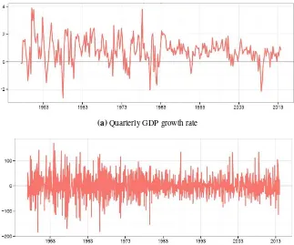
To gain insights about the time series properties of our data sets, we first plot the logarithmic changes in real US GDP and EPU, cf. Figure 1. We observe a higher variability in EPU than in real GDP growth. As is standard practice in time series econometrics, we then tested for the unit root properties of the log-levels of real GDP and the EPU index. In this regard, we used the Ng and Perron (2001) unit root test, which has been shown to have very good size and power properties, relative to other standard unit root tests. Under the assumptions of a constant, and constant and trend in the test equation, the null of unit root cannot be rejected for the levels of the series. However, first-differencing ensures that the two variables of concern (growth rate of real GDP and growth rate of EPU), are stationary. These results along with the summary statistics of the growth rates of the two variables have been reported in Table 1.
So we work with percentage changes,C, of real GDP or EPU, computed as:
Ct =100∗[ln(datat)−ln(datat−1)], (1)
wheredatat denotes the real US GDP or EPU at periodt.
(a)Quarterly GDP growth rate
(b)Monthly economic policy uncertainty index (percent change)
Figure 1: Plots of growth rates of U.S. real GDP and EPU.
3 Methodology
The recently developed MF-MS-VAR model by Camacho (2013) in state space representation can be formalized as:
Zt=Ωδtθt+εt, , t=1,2, . . . ,T, (2)
whereZt =
Ztq,′1,Ztm,2′ ′
is a vector that contains quarter-on-quarter and
month-on-month growth rates of the economic indicators,θt= Zm
is a vector of lagged month-on-month growth rates,Ωδt = (A1,A2,A3,A4,A5)is a
Block matrix whose elements are given by:
A1= the same at monthly frequency. As stressed in Mariano and Murasawa (2003) the quarter-on-quarter growth rate of quarterly indicators calculated at each month of the sample can be obtained as the average sum of previous month-on-month growth rates as follows:
Camacho (2013) assumed that the monthly growth rates of the economic indicators follow a Markov switching VAR(p) process, which is governed by a state variableδt, that is assumed to evolve according to a first-order Markov chain with transition probability:
Pr(δt = j|δt−1=i,δt−2=h, . . . ,ℑt−1) =Pr(δt= j|δt−1=i) =pi j, (6)
wherei,j=0,1 andℑt is the information set available at the timet. Using the
Kalman filter, the MF-MS-VAR model can be easily estimated via maximum likelihood method, with easily computable filtered probabilities: Pr(δt= j|ℑt), and smoothed probabilities: Pr(δt= j|ℑT). We refer the reader to Camacho (2013) for more details on the estimation procedure.
4 Empirical Results
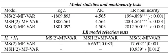
Table 2:Nonlinearity and model selection tests
Model statistics and nonlinearity tests
Model logL AIC LR nonlinearity
MS(2)-MF-VAR -1809.893 4.565 1994.898∗∗∗[<0.001]
MSH(2)-MF-VAR -1806.561 4.564 2001.561∗∗∗[<0.001]
MS(3)-MF-VAR -1801.092 4.503 2012.500∗∗∗[<0.001]
LR model selection tests
H0/H1 MS(2)-MF-VAR MSH(2)-MF-VAR MS(3)-MF-VAR
MS(2)-MF-VAR – 6.663∗[0.083] 17.602∗∗[0.001]
MSH(2)-MF-VAR – – 10.939∗∗[0.012]
Note: The table reports the the log likelihood (logL), Akaike Information Criterion (AIC), and likelihood ratio (LR) tests for homoscedastic Markov switching, MS(k), and heteroskedastic Markov switching, MSH(k), mixed frequency vector autoregression models withkregimes. The maximum upper bound of for thep-values (Davies, 1987) of the LR tests are given in brackets.∗∗∗,∗∗, and∗denote significance at 1%, 5% and 10%, respectively.
switch, since shifts do not depend on the dynamics of the autoregressive process or the covariance matrices (Hamilton, 1989). We first establish nonlinearity and perform several likelihood ratio (LR) tests in order to decide on the type of the Markov switching model. We consider both homoscedastic Markov switching, MS(k), and heteroscedastic, MSH(k), models withk=2,3 regimes. In the ho-moscedastic model, the covariance matrix of the residuals is constant across the regime, i.e.,εt∼N(0,R), and it varies with regimes in the heteroscedastic case, i.e., εt∼N(0,Rδ
t). Tests results are given in Table 2. First, the results in Table 2 show that linearity is strongly rejected against all MS models. Second, MS(2)-MF-VAR model is only rejected at 10% significance level agains the MSH(2)-MF-VAR. Third, both AIC and LR test select the three regime MS(3)-MF-VAR over the others. The smoothed regime probabilities of the MS(3)-MF-VAR model are plotted in Figure 4 in the Appendix indicate that second and third regimes both corresponds to the recession periods. Given that the second regime might indeed be a spurious regime corresponding to a few spikes in the recession periods and numerous empirical studies that only consider a two regime MS model for the business cycle analysis (see studies discussed in e.g., Hamilton and Raj, 2002) we use the two regime MS(2)-MF-VAR for the analysis in the rest of the paper.
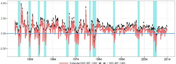
(a)Monthly indicators of quarterly real GDP growth rate
(b)Smoothed probabilities of recession regime
Figure 2: Monthly indicator of quarterly real GDP growth rate from the MS-MF-VAR model, and smoothed recession probabilities. Note: Shaded areas in panels (a) and (b) represent the recessions as documented by the NBER.
models. We also analyse and extend MF-MS-VAR model that includes inflation and 3-month treasury bill rate in addition to the economic policy uncertainty. Both indicators are in accordance with the NBER-referenced business cycles (indicated by the shaded areas in Figure 2). The positive growth rates are interrupted by large changes in the direction, which in turn, align quite well with the U.S. recessions.
the economic indicators into recession probabilities. In order to determine the accuracy of the MF-MS-VAR model to account for the business cycles, Panel (b) of Figure 2 plots the values of the smoothed recession probabilities of state δt=1. The fact that the probability of state 1 corresponds to recessions is due to the reasonable match between the quarters of high probabilities of this state and the NBER recessions. The MF-MS-VAR model is observed to capture the recessions quite well.5
Even though we observe a high correlation between the probabilities of re-cession and the NBER referenced rere-cessions, the question is whether or not the MF-MS-VAR model outperforms other possible competitors used for business cycles dating. In this regard, we look at a MS-VAR model – where the monthly EPU are averaged over three-months to produce quarterly values of the same, and a MS-AR model, as two possible competitors. We start off with in-sample accuracy, and compute the quadratic probability score (QPS) in this regard, as proposed by Brier (1950). Formally,
wherept is the forecast probability made at the timet,rt is the realization of the
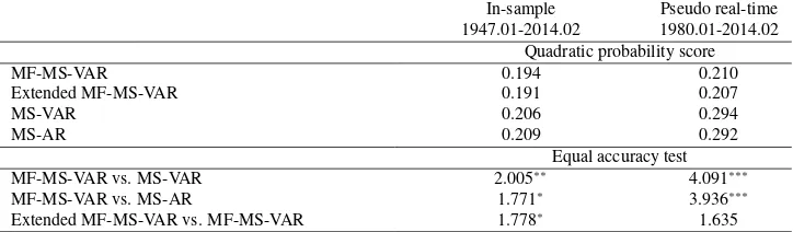
event at the timet, andT denotes the total number of the observations. We note that QPS ranges between 0 and 1, with a score of 0 indicating a perfect accuracy. The computed values of QPS for our models are near zero and reported in Table 3. The Extended MF-MS-VAR model provides the smallest score, followed by the MF-MS-VAR, the MS-VAR, and MS-AR models for the in-sample. In addition to the QPS, we also apply the equal forecast accuracy (DM) test of Diebold and Mariano (1995). When we compare the MF-MS-VAR models with the MS-VAR (MS-AR), the null of equal predictive accuracy is rejected at 5% (10%) levels of significance. So results from the QPS and the Diebold and Mariano (1995) tests highlights the superiority of the MF-MS-VAR models relative to the MS-VAR and MS-AR models, based on an in-sample analysis.
5 The results for the Extended MF-MS-VAR model are plotted in Figure 3 in the Appendix. The
Table 3:Relative performance metrics and equal forecast accuracy tests
MF-MS-VAR vs. MS-VAR 2.005∗∗ 4.091∗∗∗
MF-MS-VAR vs. MS-AR 1.771∗ 3.936∗∗∗
Extended MF-MS-VAR vs. MF-MS-VAR 1.778∗ 1.635
Note: The table reports the QPS and Diebold and Mariano (1995) equal test for mixed-frequency Markov-switching vector autoregression (MF-MS-VAR), Markov-Markov-switching vector autoregression (MS-VAR), and Markov-switching autoregression (MS-AR) models. Extended MS-MF-VAR model includes inflation and 3-month treasury bill rate in addition to the economic policy uncertainty.∗∗∗,∗∗, and∗denote significance at 1%, 5% and 10%, respectively.
However, the in-sample analysis does not account for the effect of the non-synchronous releases that characterizes the real-time flow of macroeconomic information. To provide a more realistic assessment of the reliability of MF-MS-VAR results, we also look at a pseudo real-time analysis as proposed by Camacho (2013). Towards this end, we evaluate the ability of the MF-MS-VAR models, relative to the MS-VAR and MS-AR models, in predicting recession probabilities (based on recursive estimation of the models) over the out-of-sample period of 1980:01–2014:02, using an in-sample period of 1947:1–1979:12. The decision to start our out-of-sample forecasting exercise in 1980:01, which also gives us more or less a 50 percent split of the in- and out-of-samples, is in line with a major breakpoint due to changes in US monetary and fiscal policies (see Bekiros and Paccagnini, 2013, for a detailed discussion in this regard). As can be seen from Table 3, the Extended VAR is still the best model followed by the MF-MS-VAR model,6but the MS-AR model performs slightly better than the MS-VAR
its smoothed recession probabilities are quite analogous to those of the MF-MS-VAR model and, therefore, not discussed here since our focus is the EPU.
6 Superiority of the Extended MF-MS-VAR over the MF-MS-VAR indicates that the inflation and
model, based on the QPS statistic. In addition, the Diebold and Mariano (1995) rejects the null of equal forecast accuracy of the MF-MS-VAR model relative to both the MS-VAR and MS-AR models at 1% level of significance. So, as with the in-sample, the MF-MS-VAR model outperforms its two competitors in a pseudo real-time forecasting exercise as well. Our results, hence, provides convincing evi-dence in favor of the MF-MS-VAR model in predicting U.S. recession probabilities for both within and out-of-sample exercises.
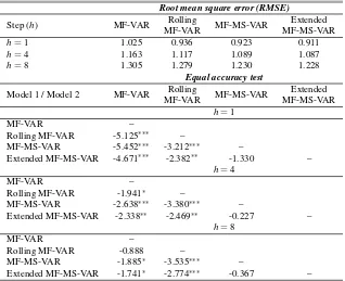
In order to gain more insight on the relative performance of the MF-VAR and MS-MF-VAR models we carry out an out-of-sample forecasting exercise over the monthly sample period 1980:1–2014:2. The out-of-sample forecast exercise uses a recursive design where the starting point of the estimation is fixed at 1947:01 for the MF-VAR, MS-MF-VAR, and the Extended MS-MF-VAR models. We also include a rolling MF-VAR model, with a fixed window size of 60, in the exercise since it better adopts to structural breaks and, therefore, more comparable to MF-MS-VAR models. The forecasts are obtained for the monthly indicators of the quarterly GDP growth rate forh=1,4,8 steps and the forecast errors are computed on a quarterly basis using the actual quarterly GDP growth rates. The out-of-sample forecasting performance of the models are compared in terms of root mean square error (RMSE). We also report the equal forecast accuracy DM tests for statistical comparison of the forecasting performances. Table 4 reports results for the out-of-sample forecasting exercise. In terms of RMSE, the results in Table 4 show that the Extended MS-MF-VAR has the best forecasting ability at all forecast horizons followed by the MS-MF-VAR model. The MS-MF-VAR models are followed by the Rolling MF-VAR and MF-VAR models, respectively. The DM tests show that the MS-MF-VAR models outperform the Rolling MF-VAR and MF-VAR models for all stepsh=1,4,8, but there is no statistically significant difference between the Extended MS-MF-VAR and MS-MF-VAR models.
5 Conclusion
Table 4:Out of sample forecast error statistics and equal forecast accuracy tests
Model 1 / Model 2 MF-VAR Rolling
MF-VAR MF-MS-VAR
Extended MF-MS-VAR -4.671∗∗∗ -2.382∗∗ -1.330 –
h=4
MF-VAR –
Rolling MF-VAR -1.941∗ –
MF-MS-VAR -2.638∗∗∗ -3.380∗∗∗ –
Extended MF-MS-VAR -2.338∗∗ -2.469∗∗ -0.227 –
h=8
MF-VAR –
Rolling MF-VAR -0.888 –
MF-MS-VAR -1.885∗ -3.535∗∗∗ –
Extended MF-MS-VAR -1.741∗ -2.774∗∗∗ -0.367 –
Note: The table reports the out-of-sample root mean square error (RMSE) and Diebold and Mariano (1995) equal forecast accuracy (DM) test for mixed-frequency vector autoregression (MF-VAR), Rolling MF-VAR, mixed-frequency Markov-switching vector autoregression (MF-MS-VAR), and Extended MF-MS-VAR. Ex-tended MS-MF-VAR model includes inflation and 3-month treasury bill rate in addition to the economic policy uncertainty. The RMSE and DM reported in the table are for forecasting the quarterly real GDP growth. The out-of-sample period covers 1980:1-2014:1. The rolling window size for the Rolling MF-VAR is 60. The DM test is calculated for the difference of the squared forecast error of Model 1 minus the squared forecast error of Model 2.∗∗∗,∗∗, and∗denote significance at 1%, 5% and 10%, respectively.
quarterly values) and MS-AR models. Our results not only highlight the importance of the monthly EPU in predicting the movements of the quarterly GDP growth rates and the associated recessionary regimes, but also shows that important information emanating from the EPU will be compromised if one averages its monthly values into quarterly ones.
Appendix
(a)Monthly indicators of quarterly real GDP growth rate
(b)Smoothed probabilities of recession regime
(a)Smoothed probabilities of regime 1
(b)Smoothed probabilities of regime 2
(c)Smoothed probabilities of regime 3
Figure 4: Smoothed recession probabilities of the three regime MS(3)-MF-VAR model. Note: Shaded areas in panels (a), (b), and (c) represent the recessions as documented by the NBER.
References
Aastveit, K. A., Natvik, G. J., and Sola, S. (2013). Economic uncertainty and effectiveness of monetary policy. URLhttp://www.norges-bank.no/pages/95985.
Alessandri, P., and Mumtaz, H. (2014). Financial regimes and uncertainty shocks.
Bai, J., and Perron, P. (2003). Computation and analysis of multiple structural change models. Journal of Applied Econometrics, 18(1): 1–22. URL http: //onlinelibrary.wiley.com/doi/10.1002/jae.659.
Baker, S., Bloom, N., and Davis, S. (2016). Measuring economic policy uncertainty. The Quarterly Journal of Economics, pages 1–37. URLhttp://qje.oxfordjournals. org/content/early/2016/07/05/qje.qjw024.abstract.
Bekiros, S., and Paccagnini, A. (2013). On the predictibility of the time-varying VAR and DSGE models. Empirical Economics, 45(1): 635–664. URL http: //link.springer.com/article/10.1007/s00181-012-0623-z.
Berge, T. J., and Jordà, O. (2011). Evaluating the classification of economic activity into recessions and expansions. American Economic Journal: Macroeconomics, 3(2): 246–277. URLhttp://www.ingentaconnect.com/content/aea/aejma/2011/ 00000003/00000002/art00009.
Bernanke, B. (1983). Irreversibility, uncertainty and cyclical investment.Quarterly Journal of Economics, 98(1): 85–106. URLhttp://www.jstor.org/stable/1885568.
Bloom, N. (2009). The impact of uncertainty shocks. Econometrica, 77(3): 623–685. URLhttp://onlinelibrary.wiley.com/doi/10.3982/ECTA6248/abstract.
Brier, G. W. (1950). Verification of forecasts expressed in terms
of probability. Monthly Weather Review, 78(1): 1–3. URL
http://journals.ametsoc.org/doi/abs/10.1175/1520-0493%281950%29078%
3C0001%3AVOFEIT%3E2.0.CO%3B2.
Brock, W., Dechert, D., Scheinkman, J., and LeBaron, B. (1996). A test for indepen-dence based on the correlation dimension.Econometric Reviews, 15(3): 197–235.
URLhttp://www.tandfonline.com/doi/abs/10.1080/07474939608800353.
Camacho, M. (2013). Mixed frequency VAR models with Markov switching dynamics. Economics Letters, 121(3): 369–373. URLhttp://www.sciencedirect. com/science/article/pii/S0165176513004175.
Colombo, V. (2013). Economic policy uncertainty in the US: Does it matter for the Euro area. Economics Letters, 121(1): 39–42. URLhttp://www.sciencedirect. com/science/article/pii/S0165176513003066.
Davies, R. (1987). Hypothesis testing when a nuisance parameter is present only under the alternative. Biometrika, 74(1): 33–43. URL http://www.jstor.org/ stable/2336019.
Diebold, F. X., and Mariano, R. (1995). Comparing predictive accuracy.Journal of Business and Economic Statistics, 13(1): 253–263.URLhttp://amstat.tandfonline. com/doi/abs/10.1198/073500102753410444.
Dixit, A. K., and Pindyck, R. S. (1994). Investment under uncertainty. Princeton: Princeton University Press.
Estrella, A., and Mishkin, F. S. (1998). Predicting U.S. recessions: Financial vari-ables as leading indicators. The Review of Economics and Statistics, 80(1): 45– 61. URLhttp://www.mitpressjournals.org/doi/abs/10.1162/003465398557320#
.WA8jz8ms2yE.
Hamilton, D. J., and Raj, B. (2002). New directions in business cycle research and financial analysis. Empirical Economics, 27(2): 149–162. URLhttp://link. springer.com/article/10.1007/s001810100115.
Hamilton, J. D. (1989). A new approach to the economic analysis of nonstationary time series and the business cycle. Econometrica, 57(2): 357–384. URLhttp: //www.ssc.wisc.edu/~bhansen/718/Hamilton1989.pdf.
Hamilton, J. D. (2008).New palgrave dictionary of economics, chapter Regime-switching models. Palgrave McMillan Ltd., 2nd edition.
Jurado, K., Ludvigson, S. C., and Ng, S. (2015). Measuring uncertainty. The American Economic Review, 105(3): 1177–1216. URLhttp://www.aeaweb.org/ articles.php?doi=10.1257/aer.20131193.
Karnizova, L., and Li, J. C. (2014). Economic policy uncertainty, financial markets and probability of US recessions. Economics Letters, 125(2): 261–265. URL
http://www.sciencedirect.com/science/article/pii/S0165176514003541.
Mariano, R., and Murasawa, Y. (2003). A new coincident index of business cycles based on monthly and quarterly series. Journal of Applied Econometrics, 18(4): 427–443. URLhttp://onlinelibrary.wiley.com/doi/10.1002/jae.695/abstract.
Mumtaz, H., and Theodoridis, K. (2016). The changing transmission of un-certainty shocks in the US: An empirical analysis. Journal of Business and Economic Statistics, pages 1–39. URLhttp://www.tandfonline.com/doi/abs/10. 1080/07350015.2016.1147357.
Mumtaz, H., and Zanetti, F. (2013). The impact of the volatility of monetary policy shocks. Journal of Money, Credit and Banking, 45(4): 535–558. URL
http://onlinelibrary.wiley.com/doi/10.1111/jmcb.12015.
Ng, S. (2014). Viewpoint: Boosting recessions. Canadian Journal of Economics, 47(1): 1–34. URLhttp://onlinelibrary.wiley.com/doi/10.1111/caje.12070/epdf.
Ng, S., and Perron, P. (2001). Lag length selection and the construction of unit root tests with good size and power. Econometrica, 69(6): 1519–1554. URL
http://onlinelibrary.wiley.com/doi/10.1111/1468-0262.00256/abstract.
Please note:
You are most sincerely encouraged to participate in the open assessment of this article. You can do so by posting comments.
Please go to:
http://dx.doi.org/10.5018/economics-ejournal.ja.2016-27
The Editor