International Review of Economics and Finance 8 (1999) 147–163
A model of bank contagion through lending
Patrick Honohan
a,b,*
aDevelopment Research Group, The World Bank, 1818 H Street NW, Washington, DC 20433, USA bCentre for Economic Policy Research, London, UK
Received 1 October 1997; accepted 22 May 1998
Abstract
While the theoretical literature on bank contagion has focused mainly on deposit withdraw-als, a disturbance on the lending side can also propagate through the system. We find that commonly observed features of banking crises can be rationalized in terms of a simple oligopoly model of bank lending. Informational externalities can result in banks over-committing to risky lending, and finding themselves in difficulties even if they were not consciously taking advantage of the deposit-put option implicitly offered by government guarantees. Liberalization of entry can also disturb an oligopolistic equilibrium and induce banks to shift to a riskier stance—this effect will be stronger if the old banks have a higher cost-base with quasi-fixed factors of production. 1999 Elsevier Science Inc. All rights reserved.
Keywords:Banking crisis; Information externalitites; Contagion
1. Introduction
When systemic banking crises strike, they may have been caused by system-wide shocks, or by a common behavioral response to perverse incentives. But the possibility that a problem in one segment of the system, or even in one institution, may propagate and infect the system more widely must also be considered.
Observers of recent banking crises have documented the herding behavior of banks with associated euphoria and overlending, which has often preceded the collapse. They have also noted the scramble for return at the cost of higher risk, as existing banks struggle to stay in business in the face of new competition in a liberalized financial market. Both of these important phenomena reflect a type of contagion that has been overshadowed by the theoretical literature that focuses on depositor runs. Indeed, the banking crises of the past quarter-century in industrial countries have
* Corresponding author. Tel.: 353-1-4911562; fax: 353-1-4065422.
E-mail address: [email protected] (P. Honohan)
been characterized more by correlated failures in credit quality than by depositor runs. The purpose of this paper is to describe how disturbances in one part of the banking system are transmitted through lending decisions. To this end, we develop a simple model of oligopolistic banking and describe the equilibrium risk of the banks’ portfolio. Small disturbances directly affecting only one bank can propagate through the system. We show in particular how the arrival of a new entrant can lead to riskier behavior by all banks, and how false information leading to over-optimism by one bank can lead to over-optimism by all.
An extensive literature has considered the structure and stability of banking systems. Banking forms a network in which a relatively small number of institutions interact to provide credit and process information (Shubik, 1990). Disturbances to part of such a network can have far-reaching and hard-to-predict consequences for the whole (Honohan & Vittas, 1997). While financial networks appear to be robust to most disturbances (Benston & Kaufman, 1995), positive feedback could cause catastrophic collapse in some circumstances. The fear of contagious propagation of disturbances through the financial system has influenced policy structures such as (on the one hand) government deposit guarantees and (on the other) the imposition and supervision of restrictive regulations on bank conduct. The degree to which contagion actually pres-ents a serious risk in practice is debated (Kaufman, 1994). While the theoretical literature on bank contagion has focused mainly on deposit withdrawals as a propaga-tion mechanism (cf. Diamond & Dybvig, 1983; Postlewaite & Vives, 1987; Chari & Jagannathan, 1988; and Calomiris & Kahn; 1991), the empirical and historical litera-ture1also mentions that a disturbance on the lending side can propagate through the
system (cf. Davis, 1992; Honohan, 1997).2
To capture some of the features of how competitive pressures on bank decision-making and risk-taking propagate, this paper considers a simple oligopoly model of bank lending. For heuristic purposes, we begin in Section 2 with an intuitive account of the model and the results obtained. We show that both the commonly observed features of herding behavior and the acceptance of increased risk as a response to increased competition can be rationalized in terms of such a model.
In the basic model, presented in Section 3, each of a small number of banks faces a downward sloping demand curve from low-risk borrowers. The slope of this curve is common knowledge and banks compete with Cournot strategies to determine their volume of lending. Banks also have an alternative high-risk lending category. Cournot competition occurs in the market for high-risk loans, too. We assume that the supply of low- and high-risk loans are independent, and that banks can identify which borrow-ers are high-risk. Banks also incur costs, not only the interest costs of deposits, but resource costs in administering, processing and monitoring. These costs will vary with the size of the balance sheet. Finally, the supply of deposits to the bank is not dependent on the risk of failure (implicitly because the deposits are regarded as being guaranteed by the unmodelled government).
We adapt this set-up to consider the effect of two distinct types of disturbance on system-wide exposure or risk of failure.
involved in the high-risk loans is imperfect, and that each bank attempts to infer the degree of risk from observation of market behavior. We show that plausible learning processes can amplify the risk of systemic failure, relative to a situation where no learning takes place. Informational externalities can result in banks over-committing to high-risk lending, and finding themselves in difficulties—even if they were not consciously taking advantage of the deposit-put option implicitly offered by govern-ment guarantees.
In Section 5, we consider the role of liberalization, modeled as new entry, in circum-stances where existing banks are locked into a certain level of resource costs; in other words, there are quasi-fixed factors of production. We show how entry, disturbing the previous oligopolistic equilibrium, will tend to increase the amount of risk borne by the system above what would occur in equilibrium. This effect will be stronger if the old banks have a higher cost base. The model suggests that the impact effect of liberalization in this regard is likely to be more severe than its long-term effect.
2. An Intuitive Account
Bank lending typically operates in an environment that is not perfectly competitive; banks deal in assets that are not priced on an open market. These are two key features that we try to capture in the modeling approach adopted in this paper. They allow us to see how changes in the environment can swing a banking system from a position of safety to one in which failure becomes likely.
In particular, the fact that the true value of assets is revealed slowly allows misinfor-mation to propagate uncorrected in the market, thereby increasing the risk of failure. Many recent studies have focused on the deposit-put: the fact that a bank offering to accept deposits that are—explicitly or implicitly—insured by the government, is only promising to pay back if it remains solvent. By manipulating the risk of failure, the bank can effectively reduce the total expected cost of servicing these deposits. In other words, through the deposit insurance, the bank has acquired a put option on the value of the deposits, an option whose value increases with the risk of bank failure. The present model also embodies a deposit put option, but it is one whose value may, in certain conditions, be zero. Changes in the competitive environment, for exam-ple new entry by a low-cost bank, may shift the existing banks from a position where failure is impossible (and the deposit-put worthless) to one where failure is a real possi-bility; the banks, therefore, may begin to exploit the deposit-put in a socially costly way. Each of the several banks in our model is seen as having unlimited access to deposits paying an exogenously fixed interest rate. (That the deposit interest rate does not depend on the risk of failure reflects the implicit assumption that deposits are being guaranteed by the unmodeled government). The banks must hold a minimum capital ratio, and they can access capital at an exogenously fixed cost, higher than that on deposits.3 They can invest their resources in loans, distinguishing between low- and
high-risk loans.4We allow for a constant per-dollar unit administrative cost of lending,
yield a known return which declines with the size of aggregate lending. The elasticity of this low-risk loan supply curve is common knowledge.
The high-risk loans pay an exogenously fixed6return if successful, but the probability
of success declines with the volume of aggregate lending. We make various assumptions about participants’ information about the elasticity of this probability of success curve. This declining probability of success is a short-hand intended to reflect an underlying reality which we can picture as beginning with the banks being faced with a pool of applicants. Some of the applicants are identifiable as low-risk. Efforts are made to screen the remainder, but (presumably because the most plausible applicants are granted loans first) the success rate of screening deteriorates as the aggregate number of loans to this category increases. We assume that the supplies of low- and high-risk loans are independent, and (as mentioned) that banks can identify which borrowers are high-risk.
We model the market equilibrium as a Cournot-type, where each bank optimizes conditional on the lending decisions of the others.7 There are thus two important
downward sloping market demand curves: that coming from low-risk borrowers and that from the high-risk borrowers. The two elasticities of these curves are determinants, along with the exogenous interest rates on deposits and capital, of the equilibrium of the system and, in particular, of the equilibrium ratio of low- to high-risk loans.
If the capital adequacy requirements are sufficiently high, we are in the no-failure zone and no bank will fail even if all of its high-risk borrowers default. If capital requirements are lower, then banks will recognize that there is a possibility of failure. Recognizing that this gives them the possibility of exercising the deposit-put, they will increase the share of high-risk loans, thereby increasing the probability of failure. The precise conditions under which this occurs are spelled out in the next section. So far, nothing has been said about contagion as such (in particular, a bank can be in the failure zone with no contagion existing).
This basic framework is then used to explore the consequences of informational disturbances and entry. Up to now, we have assumed that the banks know the two market demand curves. Each bank may have some imperfect information, and this will provide an incentive for all to observe each others’ behavior in order to try to infer what the others know. This kind of problem is widely discussed in connection with the determination of market prices of assets when information is imperfect and unevenly distributed. In that case, a key question is the degree to which all of the information in the market becomes revealed in prices. But here the assets are not priced, so that information does not feed back directly onto market prices.
optimism by one bank can result in too much risky lending throughout the system. That certainly rings true for the kinds of bandwagon effect or herd behavior observed in credit-sustained property booms.
The effects of entry can also be modeled as a disturbance to the Cournot equilibrium. Here, the interesting point is that the arrival of a new bank can move the equilibrium out of the no-failure zone, leading not only to a risk of failure, but to the exploitation of the deposit-put and increasingly risky behavior. The problem is that, having inherited staff levels that justify a certain scale of lending, incumbents will treat these as sunk costs and continue to lend at a level which is beyond what is now prudent, given the lower returns and higher risk that is emerging in the market as a result of the arrival of the new entrant.
In the long-run, when the fixed costs incurred by the old banks are no longer relevant, it is possible that the system could return to the no-failure zone. To that extent, the disturbing effect of entry may vanish over time, and this disturbance may well be an acceptable cost to pay for a more efficient long-term equilibrium.
3. The Basic Model
To begin, we describe those features of the set-up that are common to both variants of the model. There are n banks in the market. Each bank i can access deposits at an exogenously fixed return r0 (interest rate r0 2 1). It can supply loans at a
per-dollar unit administrative cost wi. There are two types of loan: low- and high-risk.
The low-risk loans (risk-free loans) yield a certain return rL. Each bank’s portfolio
of high risk loans yieldsrHif repaid, nothing otherwise. The probability of repayment
is denotedu. We assume this risk is non-diversifiable; the entire risky portfolio of a given bank either repays or does not.8The opportunity cost of capital is exogenously
fixed atrC. It is assumed that the maximum yield on a high-risk loanrHis exogenously
fixed, but the low interest yieldrLand the probability of repaymentu depend on the
aggregate volume of loans of each type. We writexiand zi,XandZ, as the quantity
of low-risk and high risk loans of bankiand the aggregate of the banks respectively. Thus the dependence of the returns on volume is: rL 5 f (X) and u 5 g (Z) with
elasticities:e 5 Xf9(X)/rLand h 5 Zg1(Z)/u.
Banks are required to hold a minimum capital-to-assets ratio of g, and we will assume that the ex ante franchise value of banking is sufficient to remunerate this capital, but that the opportunity cost of capitalrCis higher thanr0so that the minimum
capital ratio is binding. The weighted average cost of funds is thus [Eq. (1)]:
r* 5(1 2 g)r0 1 grC. (1)
3.1. Equilibrium in the no-failure zone
If the capital requirement is set sufficiently high so that the probability of failure is zero in the relevant range—in other words if we are in the “no-failure zone”—then the appropriate maximand is:
Maximization of the expected value of Eq. (2) by each bank under the Cournot assumption that the volume decisions of the others are not sensitive to one’s own, leads to the familiar Lerner price-cost ratio conditions for each bank in the two markets:
The intuition here is that each bank takes into account the impact of its own lending on the rate of return; thus it will expand its lending only to the point where, conditional on the lending of all other banks, a further increase would lower the gross margin on other loans by more than it would generate in new net revenue. These conditions Eqs. (3) and (4) can thus be seen as reaction functions9determining each bank’s loan
supplyxiandzias a function of the lending by others: (X2xi) and (Z2zi). Aggregating
these over all of the banks provides the market equilibrium conditions:
12r*X1 S wixi
The market equilibrium conditions Eqs. (5) and (6) thus determine the risk-free (low-risk) lending rate rL and the risk parameter u. In the case where all banks are
identical, the sum of squared market shares (Herfindahl index) is simply the reciprocal of the number of banks, so the market equilibrium conditions reduce to [Eqs. (7) and (8)]:
12r* 1w
In words, oligopolistic competition between the banks will drive loan supply up to the point where the expected profit margin, as a percentage of gross return on each sub-portfolio, is inversely proportional to the price elasticity of the loan supply. These conditions are, of course, directly analogous to classic IO results defining the profit share as directly proportional to the absolute value of the elasticity of demand and inversely proportional to the number of firms.
A small number of banks and a high capital requirement means that the gross return on low-risk assets is high: writing the interest and administrative costs devoted per dollar of lending as:
we may regard the gross profit per dollar lent rL2b
ias a measure of the franchise
value of low-risk banking.
3.2. Equilibrium in the failure zone
If the capital adequacy requirements are not sufficient to rule out failure, then the optimization criteria change. This is because, by increasing the share of high-risk loans in its portfolio, each bank can influence the value of the deposit-put, the possibility that losses by the bank in excess of its capital (thereby threatening the depositors) will be met by the government.
If the high-risk loan is not repaid, then the government may have to pay out to depositors. The government is at risk of having to make such a pay-out if the sum due to the depositors and factors of production (the latter assumed already paid out of depositor funds) exceeds the amount received by the bank from the low risk borrowers, i.e. the government is at risk if Condition F holds, defined by the inequality
bi(xi1zi) 2rLxi;Fi.0.
As the deposit-put will only have value if this inequality is satisfied, we say that a bank is ex ante in the failure zone whenever Condition F holds. Fiis effectively the
value of the deposit put if exercised. If Condition F does not hold, then the bank will still be able to pay depositors even if the high-risk loan is not repaid; it is not in the failure zone, and the deposit put has no value.
Note that Condition F will not hold if what we have termed above the franchise value of low-risk banking (rL2 b
i) is sufficiently high.
The bank maximizing expected profits in the failure zone will thus maximize [Eq. (9)]
pi1 (1 2 u)Fi5 u rHzi1 rLxi2(r* 1wi) (xi1zi)
1(1 2 u)[bi(xi1zi) 2rLxi]
5 u (rHz
i1rLxi)2 (u bi1 grC)(xi1zi).
5 u (rHz
i1rLxi) 2 u(r* 1wi1a) (xi1zi) , (9)
where,
a 5 grC(1 2 u)/u
In examining this expression it is worth noting that, in a failure zone, the shareholders of a failing bank can lose their entire capital, including the profit from the low-risk loans. On the other hand, from the bank’s (shareholder’s) viewpoint the costs, other than opportunity cost of capital, also become contingent on not failing. Although the precise formulation is an implication of the very simple dichotomous risk specification, the insight that the risk differential between the two loan categories is reduced seems robust. An increase inu therefore affects the expected return not only on the high-risk asset, but also on the low-high-risk asset and the effective cost of lending.
12r* 1wi1a
modifies the mark-up ratio, and is a grossed-up risk asset quantity, effectively taking account of the increased risk of failure, and
z*i 5 zi1
hence of losing the profits from the risk-free asset, imparted by additional purchases of the high-risk asset.
The only difference between Eq. (3) and Eq. 1(0) is that the cost term in Eq. (10), i.e. r* 1 wi 1 a, is evidently larger than that in Eq. (3). Thus the existence of the
deposit-put acts just like an increase in the cost of capital.
The relation between Eq. (4) and Eq. (11) is more complex. The factorBiby which
the LHS of Eq. (11) differs from that of Eq. (4), tends to zero for small capital requirements (g → 0) making the LHS of Eq. (11) larger than that of Eq. (4). Accordingly, the grossed-up risk assets total is higher than the total satisfied:
zi,z*i ,zi1 xi.
Comparing the incentives of an individual bank in the failure zone with that of the same bank not in the failure zone, conditional on market pricesrLandu, we see that
the failure zone bank will place slightly less in low-risk assets. Furthermore, its grossed-up risk position,z*i, will be higher provided thatBi,1; and the net amount placed
in high-risk assets, zi, will also be larger, unless what we have termed the franchise
value of low-risk banking is sufficiently high. The condition10 under which the bank
will place more in high-risk assets will be referred to as Condition R.
The market equilibrium condition for identical banks in the failure zone is a straight-forward aggregation of Eq. (10) and Eq. (11). Therefore, for the same elasticity e, the equilibrium low-risk rate rLis unambiguously higher, though by a small amount
if capital requirements g are small. Equilibrium in the high-risk asset market will involve (if elasticityhis little changed and under condition R) increased lending and lower probability of successu.
i. an increase in the low-risk lending rate sufficient to offset the relatively higher burden being borne by the capital committed to “low-risk” lending, but which will be lost if the bank fails;
ii. an expansion of high risk loans, to the point where the value of u has fallen sufficiently to ensure that urH gives the same margin over the lower effective
marginal cost of lending.
Note that we have not yet discussed the question of contagion, to which we now turn.
4. Informational Disturbances
In this section, we assume that the banks do not knowh, but make inferences about it from (a) observing a noisy private signal and/or (b) observing the behavior of other banks in response to their noisy private signal. Because the market price of high-risk loans does not adjust (the probability of loss adjusts, but this is not observed) the learning process is rather different to that analyzed in models of learning and price revelation in securities markets.
We analyze a Cournot equilibrium of quantities and expectations, in which all banks share common information. In order to obtain closed solutions in a stochastic environment, we use a log-linear functional form for the dependencegof loss probabil-ity on the volume of lending. Specifically, we assume that [Eq. (12)]:
u 5 exp{2b Z} (12)
which implies that the absolute value of elasticityhincreases with total lending Z:
h 5 2b Z.
The parameter b is not known, but that banks have probabilistic beliefs about it represented by a Normal (Gaussian) distribution with mean zand variance s2.
We begin by examining the equilibrium behaviour conditional on the banks’ beliefs; we will return below to the determination of these beliefs. Thus, givenzands[Eq. (13)]:
%u5 (2 1 s2Z2/2) exp{2zZ}. (13)
Maximizing the expected value ofp* using this expression for the expected value ofuleads to the choice of zibeing determined by:
1 2r* 1wi
%urH 5
zi
Zh* (14)
where [Eq. (15)],
h* ; Z
%u
d%u
dZ 5 2zZ1 n (15)
and [Eq. (16)],
n 5 (zZ1 2) s
2Z2/2
In words, the equilibrium mark-up condition has the same general form as in the certainty case, but with the expected loss rate replacing the known loss rate, and with a “risk-adjusted elasticity factor” replacing the known elasticity. The risk-adjusted elasticity factor differs from the expected value of the elasticityzZby a term roughly proportional to the variance s2of the estimate of the parameter b.
Note that the individual bank condition Eq. (14) implicitly defines an zi as an
invertible function ofz, since the left hand side is a decreasing, and the right hand side an increasing, function ofz.
In the failure zone, where loss will result in failure and the deposit-put, we substitute an expression like Eq. (11) for Eq. (14) again modified by replacing u with %u and
hwith h*.
The market equilibrium condition is immediately [Eq. (17)]:
12r* 1 Swi
%urH 5 2
o
zi
Zh* (17)
It follows that an increase in uncertaintysreduces the absolute value of the risk-adjusted elasticity term so that, for the same expected value of the parameterb, the mark-up will be smaller. (This is a small effect which depends on the non-linear manner in which the parameter b enters the decision rule; it is dependent on the chosen functional form forg and might not be very robust to alternative functional forms). We turn now to the formation of beliefs concerningb. Suppose that all the banks share the same subjective variance s of the parameter b, and that this is constant. Since this is a one-period model, there is no chance for banks to update their beliefs on the basis of loan outcomes. But if the banks can observe the choicezjand the cost
levelwjof each of the other banksjthen each bank is able to infer the value of each
other bank’s zby solving the individual optimization formula Eq. (14).
For example, if it is common knowledge that each bank observes a private signal
ziwith the property that:
zi5 b 1 ui
where the ui are independent normally distributed with zero mean and a common
variancens2, then if each bank can observe what the others would lend on the basis
of their private information, then each bank can learn about the private signals and each can form the improved estimate z 5 SzI/n ofb with variance s2. Accordingly,
a configuration in which all banks do not optimally use this improved estimate cannot be an equilibrium. Specifically, each bankiwill combine its own informationzIwith
the observedSj?izj/nfor the others, a process consistent with equilibrium at a common
value z 5 SzI/n.
The restrictive nature of the Cournot assumption is relevant here in two respects. First, it implies no strategic signaling behavior. Second, it begs the question of dynamics: would a process of learning each other’s signals converge to full revelation?
be observed. Suppose that each bankiupdates its parameter valuezIweekly, beginning
with its private signalz0
i, and then (as it observes the parameterszjof others) updating
by linearly combining the last period’s parameterzt21
i with this week’s mean of other
banks’ revealed parameters, and then iterating weekly on this updating procedure.11
That is,
zt i5 g
1
n
o
zt21
j 1(12 g)zti21
It can readily be shown that this process will converge to the mean of the private signals with probability one, as the eigenroots of the associated transition matrix have
n21 roots equal to 1 2 g, and one root at unity.
In contrast to models of price signal aggregation like that in Diamond and Verrechia (1981), here the increased loan supply does not reflect back onto an observed market price until after the lending has occurred. Learning is not corrected by a global market feedback. That implies that false signals can result in banks unwittingly exposing themselves to a high risk of failure. In this case, therefore, failure can occur even if banks have not employed the deposit-put modification of Eq. (9). Furthermore, this signal propagation, along with the oligopolistic market equilibrium behavior, implies that a false positive signal received by one bank will result in all banks adopting a riskier strategy and an increase in the failure probability of banks other than the one which received the signal.
It is worth stressing again that the Cournot assumption means that each bank neglects the impact of its behavior on the others. Insofar as an expansion of risky lending in fact induces more risky behavior all around, alternative strategic assump-tions, perhaps damping the system’s response to extreme drawings of the signal, could be explored. Note also that, while we have shown how false signals could propagate, our model does not predict any amplification effect. For such an effect to occur, one would have to make additional assumptions, for example, a feedback from the increasing price of property to the assumed profitability of property loans.
5. The Effects of Entry
This section considers a two-period version of the model, where banks commit to a particular minimum level of resources at the outset, believing that both periods will be the same. However, entry occurs during before the second lending period, and we wish to examine the response of the old banks to entry.
The story here is somewhat simpler than in the previous section. Looking first at the identical banks’ case, the entry of some new banks after the first period alters the equilibrium conditions Eq. (7) and Eq. (8), lowering the margins available in both markets. This potentially drives banks into a failure regime where they are optimizing on the deposit-put.
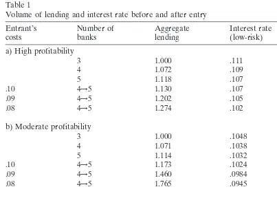
Table 1
Volume of lending and interest rate before and after entry
Entrant’s Number of Aggregate Interest rate
costs banks lending (low-risk) Lerner index
a) High profitability
3 1.000 .111 .100
4 1.072 .109 .080
5 1.118 .107 .067
.10 4→5 1.130 .107
.09 4→5 1.202 .105
.08 4→5 1.274 .102
b) Moderate profitability
3 1.000 .1048 .045
4 1.071 .1038 .036
5 1.114 .1032 .030
.10 4→5 1.173 .1024
.09 4→5 1.460 .0984
.08 4→5 1.765 .0945
c) Low profitability
3 1.000 .1025 .024
4 1.068 .1020 .019
5 1.119 .1016 .016
.10 4→5 1.212 .1009
.09 4→5 2.017 .0954
.08 4→5 2.864 .0898
each decides its decision with knowledge of the presence of others, and each therefore curtails its volume of lending. But the unanticipated arrival of a newcomer leaves the existing banks with excess capacity that they will nevertheless employ, given that they have already committed to the resources, which they now treat as sunk costs. The newcomer will not lend as much as it would have had it been in at the start, but (since the others do not contract) its increment will bring total lending above the level it would have reached had all joined at the same time, with a greater risk of driving the old banks into the failure zone.
A further twist occurs if the new entrant has lower unit costs than the incumbents. Depending on the pre-existing profit margins, a new entrant with lower cost could optimally choose a very large scale of operations, driving the old banks into a loss-making position, even on the low-risk loans. (In practice, the cost story would likely be more complex. In order to respond to the entrant, the incumbent might have to increase its own cost base, bidding more aggressively for funds and borrowers, to retain skilled staff, for advertising and so on. This kind of pressure might make the incumbent vulnerable to acquisition, a possibility not modeled here).
the demand functionsf and g. Specifically, for Table 1 we setf 5g, (so thatxi5zi)
and, assuming a negative exponential demand function,12we compute the equilibrium
of the system under optimization of the “no-failure zone” type for 3, 4 and 5 banks, and separately for the equilibrium after a fifth bank enters a four-bank system with sunk costs. The three panels are for different levels of pre-entry profitability (Lerner index), determined by the gap between assumed unit costs and the intercept of the demand function.13 For the new-entry case, we show three different sub-cases: the
first of these has the entrant’s costs at the same level as the incumbents (0.10); the other two sub-cases have lower entrant costs.
Note the large market share taken by the new entrant, and the corresponding sharp decline in the low-risk lending rate, especially when the entrant has low costs and the old profit margin (Lerner index) was low.
These calculations are based on “no-failure zone” optimization. If the old banks move into the failure zone, then the previous discussion showing the likelihood (Condi-tion R) of a shift towards high-risk lending applies.
If, on the other hand, the entry does not move the old banks into the failure zone, what can be said about the impact on the mix of low- and high-risk loans? In the present model, this hinges entirely on the behavior of the two elasticitieseand h. If these are the same, then the share of high-risk assets will not change with the overall expansion of loan business.
Thus, from the equilibrium conditions Eqs. (5) and (6), where thewi for the old
banks are understood to be the new opportunity cost of the factor resources, and whereHis the Herfindahl index, we deduce that
rL
urH5
1 1 hH
11 eH
It can be deduced that ifurH.rL(equivalently2h . 2e), the difference increases
with rising values ofH. New entry will normally lower the Herfindahl index. Accord-ingly, in this plausible case, where the expected return on high-risk loans declines more rapidly with aggregate loan volume than does the equilibrium return on low-risk loans, the new equilibrium will involve a lower expected return for high-low-risk loans, implying a relative shift in lending towards high-risk loans.
In the extreme long run, the fixed costs incurred by the old banks are no longer relevant. Then the row showing the long-run equilibrium with five banks is the relevant one. It is clear that aggregate lending is much lower than in the rows showing the impact effect of the fifth bank entering. It is even possible that the system could return to the no-failure zone. These calculations thus illustrate how the disturbing effect of entry may be larger in the short run.
6. Concluding Remarks
failure problems throughout the system. New entry tends to increase risk-taking and vulnerability to failure of the old banks, especially if they are less cost-efficient than the entrant. Optimistic signals can propagate through the system leading to increased risk of failure even where banks are not exploiting the option value provided them by deposit insurance.
The model provides a coherent theoretical underpinning for much of the recent policy discussion of systemic failure in banking. It can readily be applied or reinter-preted for other disturbances, such as the impact of an insolvent but not yet illiquid bank, or the consequences of taxation of bank intermediation.
Though the model is too simplified to be directly applicable to empirical testing, there are several striking implications that could be borne in mind for empirical work. For example:
• The moderating influence on risk-taking of franchise value measured, as has been suggested above, by the gross return on low-risk lending could potentially be identified in cross-section analyses of banking systems in different countries, or in a time series sufficiently long to show some variance in franchise value thus measured.
• The contagious flow of information through the different participants in the banking market could be empirically analyzed given bank-by-bank data on the share of lending to higher risk areas such as commercial property.
• The dynamic pattern, whereby the predicted increase in risk behavior following new entry is only temporary, appears to be novel, and could be tested.
We find that a high franchise value for low-risk banking may keep banks away from the failure zone, and even if it is not high enough to do that, it may prevent the bank’s behavioral response to failure zone behavior from increasing risk. This is consistent with standard prescriptions that call for high capitalization, and also with the idea that limiting entry reduces the risk of bank failure. However, the discussion has not been explicitly couched within a policy framework; therefore it would not be wise to jump to over-hasty policy conclusions. Even if bank entry can destabilize existing banks, that is not a sufficient reason to block entry. Other solutions can be considered: strong supervision may counter the tendencies noted and entry through acquisition may be less disruptive.
Acknowledgments
This research was commenced during a stimulating stay at the Research Department of the International Monetary Fund, for whose hospitality I am grateful.
Notes
2. Reference should also be made to the many models of individual bank behavior, e.g. Guttentag and Herring (1986) and Keeley (1990), to mention two contrasting contributions. A different strand is the macroeconomic financial crisis literature, e.g. Fisher (1933), Mankiw (1986) and Minsky (1995). Models of noise transmis-sion in securities markets have been developed, e.g. by de Long et al. (1990a,b). 3. Clearly, there would be some variation in the cost of capital with the risk assumed; this is neglected here for simplicity. Unless the required capital is very high, the variation would be of second-order importance for determining equilibrium behavior.
4. Insofar as the banks can tell whether a loan is low- or high-risk, we are abstracting from the adverse selection issue stressed in the literature, following Stiglitz and Weiss (1981).
5. In reality, no doubt, such costs are higher for high-risk loans, but we retain equal cost for simplicity. (We could also add a fixed cost component without altering the marginal conditions.)
6. Reflecting the existence of only one distinguishable risk-category.
7. For other applications of the Cournot model to banking see Honohan and Kinsella (1982), Steinherr and Huveneers (1994) and Freixas and Rochet (1997, pp. 59–61).
8. The assumption of non-diversifiability is essential, but the dichotomous pattern of returns is made for simplicity, and could be modified at the expense of additional complexity. For example, we could alternatively assume that the stochastic amount repaid on the risky portfolio was uniformly distributed on [0, 2urH]. In
that case, the expected return would still beurH, so that the equilibrium
condi-tions Eqs. (7) and (8) below for the non-failure zone would still follow. Also, the probability of failure, under Condition F, would still be a function ofu, but now it would be inversely proportional to u, instead of being equal to 12 u. Therefore the equilibrium conditions Eqs. (10) and (11) would be somewhat different, though leading to qualitatively similar conclusions.
9. Bearing in mind the dependence of the rate of return on total lending through the functions f and g.
10. The condition can be expressed as:
rH2(r*1 w
For low capital requirements, the left hand side is the ratio of the profitability of repaid high-risk loans to what we have called the franchise value of low-risk banking; the left hand side is the average profit rate on high risk loans, multiplied by the market share multiplied by the elasticity.
11. This kind of updating is a special case of those discussed by Sargent (1993). 12. Specifically:rL512 aexp(2bX). The results are not qualitatively very sensitive
to different values of the parameterb, as the equilibrium responds to changing
13. The parameters areb 5 0.3;r*1 w21 50.1 (cost for old banks);a 5 0.15 (high profitability), 0.12 (medium profitability), and 0.11 (low profitability). The Lerner index in the table is expressed as a proportion of interest rate, not of gross interest factor as in the theoretical development.
References
Benston, G. J., & Kaufman, G. G. (1995). Is the banking and payments system fragile?Journal of Financial Services Research 9, 209–240.
Calomiris, C. W., & Gorton, G. (1991). The origins of banking panics: models, facts, and bank regulation. In R. G. Hubbard (Ed.),Financial Markets and Financial Crises. Chicago, IL: University of Chicago Press.
Calomiris, C. W., & Kahn, C. M. (1991). The role of demandable debt in structuring optimal banking arrangements.American Economic Review 81, 497–513.
Chari, V. V., & Jagannathan, R. (1988). Banking panics, information and rational expectations.Journal of Finance 43, 749–760.
Davis, E. P. (1992).Debt, Financial Fragility and Systemic Risk.London: Oxford University Press. De Long, J. B., Shleifer, A., Summers, L. H., & Waldmann, R. J. (1990a). Noise trader risk in financial
markets.Journal of Political Economy 98, 703–738.
De Long, J. B., Shleifer, A., Summers, L. H., & Waldmann, R. J. (1990b). Positive feedback investment strategies and destabilizing rational speculation.Journal of Finance 45, 379–395.
Diamond, D. W., & Dybvig, P. H. (1983). Bank runs, deposit insurance and liquidity.Journal of Political Economy 91, 401–419.
Diamond, D. W., & Verrecchia, R. E. (1981). Information aggregation in a noisy rational expectations model.Journal of Financial Economics 9, 221–235.
Fisher, I. (1933). The debt-deflation theory of great depressions.Econometrica 1, 337–357. Freixas, X., & Rochet, J.-C. (1997).Microeconomics of Banking.Cambridge, MA: MIT Press. Gorton, G. (1988). Banking panics and business cycles.Oxford Economic Papers 40, 751–781.
Guttentag, J. M., & Herring, R. J. (1986). Disaster myopia in international banking.Princeton Essays in International Finance 164.
Honohan, P. (1997). Banking system failure in developing and transition countries: Diagnosis and predic-tion.Bank for International Settlements Working PaperNo. 39, and at //www.bis.org.
Honohan, P., & Kinsella, R. P. (1982). Comparing bank concentration across countries. Journal of Banking and Finance 6, 255–262.
Honohan, P., & Vittas, D. (1997). Bank regulation and the network paradigm. In H. Wolf (Ed.), Contempo-rary Economic Issues 5: Macroeconomic Policy and Financial Systems. Proceedings of the 1995 World Congress of the International Economic Association.London: Macmillan.
Kaufman, G. G. (1994). Bank contagion: a review of the theory and evidence. Journal of Financial Services Research 8, 123–150.
Keeley, M. C. (1990). Deposit insurance, risk and market power.American Economic Review 80, 1183– 1200.
Mankiw, N. G. (1986). The allocation of credit and financial collapse.Quarterly Journal of Economics 101, 455–470.
Minsky, H. P. (1995). Financial factors in the economics of capitalism.Journal of Financial Services Research 9, 197–208.
Mishkin, F. S. (1991). Assymetric information and financial crises: A historical perspective. In R. G. Hubbard (Ed.),Financial Markets and Financial Crises. Chicago, IL: University of Chicago Press. Park, S. (1991). Bank failure contagion in historical perspective. Journal of Monetary Economics 28,
271–286.
Sargent, T. J. (1993).Bounded Rationality in Macroeconomics.London: Oxford University Press. Shubik, M. (1990). A game theoretic approach to the theory of money and financial institutions. In B.
J. Friedman & F. H. Hahn (Eds.),Handbook of Monetary Economics I. Amsterdam: North Holland. Steinherr, A., & Huveneers, Ch. (1994). On the performance of differently regulated financial institutions: