www.elsevier.nlrlocaterjappgeo
Use of block inversion in the 2-D interpretation of apparent
resistivity data and its comparison with smooth inversion
A.I. Olayinka
a,),1, U. Yaramanci
ba
Department of Geology, UniÕersity of Ibadan, Ibadan, Nigeria
b
Department of Applied Geophysics, Technical UniÕersity of Berlin, Ackerstr. 71-76, D-13355 Berlin, Germany
Received 10 May 1999; accepted 19 May 2000
Abstract
The ability of a block inversion scheme, in which polygons are employed to define layers andror bodies of equal resistivity, in determining the geometry and true resistivity of subsurface structures has been investigated and a simple strategy for deriving the starting model is proposed. A comparison has also been made between block inversion and smooth inversion, the latter being a cell-based scheme.
Ž .
The study entailed the calculation by forward modelling of the synthetic data over 2-D geologic models and inversion of the data. The 2-D structures modelled include vertical fault, graben and horst. The Wenner array was used.
The results show that the images obtained from smooth inversion are very useful in determining the geometry; however, they can only provide guides to the true resistivity because of the smearing effects. It is shown that the starting model for block inversion can be based on a plane layer earth model. In the presence of sharp, rather than gradational, resistivity discontinuities, the model from block inversion more adequately represents the true subsurface geology, in terms of both the geometry and the formation resistivity. Field examples from a crystalline basement area of Nigeria are presented to demonstrate the versatility of the two resistivity inversion schemes.q2000 Elsevier Science B.V. All rights reserved.
Keywords: Resistivity inversion; Fault; Graben; Horst; Wenner array; Nigeria
1. Introduction
With the development of multi-electrode re-sistivity array, the collection of 2-D rere-sistivity data is becoming increasingly popular for
hy-)Corresponding author.
Ž
E-mail addresses: [email protected] A.I.
. Ž .
Olayinka , [email protected] U. Yaramanci . 1
Formerly at Department of Applied Geophysics, Tech-nical University of Berlin, Ackerstr. 71-76, D-13355 Berlin, Germany.
drogeological, environmental and geotechnical
Ž .
purposes Griffiths and Barker, 1993 . Although data collection is straight forward, the interpre-tation of the data can be difficult, due to the influence of equivalence, the robustness of the inversion algorithm and the number of layers or bodies used to model the data. Commercially available software applications are now rou-tinely employed for inversion of 2-D apparent resistivity data. These programs can be classi-fied into two groups, namely, smooth inversion and block inversion. Smooth inversion is a
0926-9851r00r$ - see front matterq2000 Elsevier Science B.V. All rights reserved. Ž .
cell-based inversion while in block inversion polygons are employed to define layers andror bodies of equal resistivity. The ability of these two inversion schemes in defining the geometry and true resistivity of subsurface structures, in the case where the resistivity increases with depth, is examined in this work. Typical 2-D geologic models investigated include vertical fault, graben and horst. These represent com-mon targets in groundwater and environmental investigations in areas underlain by crystalline basement rocks.
A parallel can be drawn between smooth and block inversion schemes, for the 1-D and 2-D cases. In the classical approach to the 1-D inter-pretation of vertical electrical sounding data, it is tacitly assumed that the subsurface comprises
Ž .
a small often less than 5 number of layers
ŽKoefoed, 1979; Inman, 1985; Simms and
Mor-.
gan, 1992; Muiuane and Pedersen, 1999 . This, in essence, is a highly over-constrained problem and is analogous to a block inversion scheme in the 2-D case. On the other hand, in the approach
Ž .
popularized by Zohdy 1974, 1989 , the model is overparameterized, with the number of layers in the interpreted model being equal to the number of electrode positions on the sounding curve. Such a strategy would produce a smooth model and has been extended to the
interpreta-Ž
tion of 2-D data Barker, 1992; Loke and Barker,
.
1995 .
An example of a smooth 2-D inversion
algo-Ž .
rithm is RES2DINV by Loke and Barker 1996 , while the program RESIX IP2DI by Interpex
Ž1996. is representative of a block inversion scheme. While the program RES2DINV is fully automatic, RESIX IP2DI requires that the inter-preter prescribes an initial geological model as part of the input. This starting model is ex-pected to be very close to the true model. In real cases, however, the true model is rarely, if ever, known precisely. It is demonstrated in this work that such a starting model could be based on a plane layer earth model. This simple approach has the added advantage that only the depth to
Ž .
the interface s need be varied as the inversion
result is, for all practical purposes, not depen-dent on the resistivity contrast in the starting model. With the procedure, more than one model
Žfor varying depths to the interface in the initial
.
model is produced which fit the same set of measured data. Some idea is thus provided of the range of 2-D equivalence.
The interpretation procedure described for block inversion is particularly suitable for the inversion of apparent resistivity pseudosection data from tropical and subtropical areas under-lain directly by crystalline basement rocks. Apart from a thin soil cover which may not be well-resolved in 2-D surveys because of the rela-tively large electrode spacings used, a gener-alised vertical section in such areas comprises a
Ž
low resistivity saprolite derived from the in situ
.
chemical weathering of the basement rocks
Ž
overlying a more resistant bedrock Carruthers
.
and Smith, 1992; Hazell et al., 1992 . The block inversion process then invariably involves map-ping the deviation of the true subsurface geol-ogy from the horizontal layering assumed in the starting model. Field examples from Nigeria are presented to demonstrate the usefulness of block inversion in interpreting real data.
2. Outline of method
2.1. Forward modelling of apparent resistiÕity
pseudosection data
The apparent resistivity pseudosection data were generated by a 2-D forward modelling
Ž .
program, RESIX IP2DI, by Interpex 1996 . The program uses a finite element approach to solve for the potential distribution due to point sources of current, and the potential distribution is converted into apparent resistivity values. The modelling routine accounts for 3-D sources
Žcurrent electrodes in a 2-D material model..
This implies that the resistivity can vary
arbi-Ž .
trarily along the line of surveying x-direction
Ž .
have an infinite perpendicular extension along
Ž .
the strike y-direction . In all cases of the
syn-thetic data, a layout with 81 electrodes was modelled with the Wenner array. The X- and
Z-spacings are normalized with respect to the
minimum electrode spacing A. In order to re-duce the number of model parameters to be considered, the theoretical data have been lim-ited to a single resistivity contrast of 1:20 be-tween the overburden and the bedrock. Tests with several models indicate that the forward modelling program does not contain any sys-tematic error. Moreover, the results are in agree-ment with those from another program
Ž .
RES2DMOD Loke and Barker, 1996 , which uses a finite difference method for the forward modelling.
Gauss distributed random noise with a stan-dard deviation of 5% was added to the calcu-lated responses for all the models in order to simulate field conditions. The synthetic appar-ent resistivity data were then inverted using a smooth and a block inversion scheme, respec-tively.
2.2. Smooth inÕersion
Ž
The program RES2DINV Loke and Barker,
.
1996 was employed for the smooth inversion. A forward modelling subroutine is used to cal-culate the apparent resistivity values, and a non-linear least-squares optimisation technique
Ž
is used for the inversion routine DeGroot-Hedlin and Constable, 1990; Loke and Barker,
.
1996; Dahlin and Loke, 1998 . The 2-D model used by the inversion program consists of a number of rectangular blocks whose arrange-ment is loosely tied to the distribution of the datum points in the pseudosection. The distribu-tion and size of the blocks are automatically generated by the program so that the number of blocks do not exceed the number of datum points.
The inversion routine uses the Gauss–New-ton method for a smoothness-constrained least-squares inversion, for which by default the
ver-tical and horizontal smoothness constrains are
Ž .
the same DeGroot-Hedlin and Constable, 1990 . The smoothness constrain increases with 10% per layer, which along with increasing layer thickness reduces the resolution with depth. The inversion is based on an analytical calculation
Ž .
of the sensitivity matrix Jacobian matrix for a homogeneous halfspace and the sensitivity ma-trix is re-calculated using the finite element method at each step of the iteration. The
optimi-Ž .
sation equation Ellis and Oldenburg, 1994b can be represented as :
JTJqlCTC p sJTg ylCTC r
Ž .
1Ž
i i i.
i i i i iy1where Ji is the Jacobian matrix of partial derivatives, JiT represents the transpose of J gi, i
is the discrepancy vector which contains the difference between the logarithms of calculated and observed apparent resistivity values, p isi
the perturbation vector to the model parameters,
Ž .
li is a damping factor or Lagrange multiplier used to reduce the amplitude of p , C is ai flatness-filter matrix used to minimize the roughness of p . The second term on the right-i
Ž .
hand side of Eq. 1 applies the smoothness constraint directly on the model resistivity vec-tor, riy1. This guarantees that the model will be
Ž
smooth subject to the damping factor used Ellis
.
and Oldenburg, 1994b . It also reduces the os-cillations in the model resistivity values.
2.3. Block inÕersion
The interactive program RESIX IP2DI by
Ž .
Interpex 1996 was employed for the block inversion. This is a finite element forward and inverse modelling program that calculates the
Ž
resistivity responses of 2-D earth models Rijo,
.
1977; Petrick et al., 1977; Pelton et al., 1978 . A finite element mesh is generated; each rectan-gular element is divided into four triangles and the resistivity of each triangle under the elec-trode spread is defined from the properties of the polygons which make up the model. The
Ž
Fig. 1. Schematic representation of the input model in the block inversion algorithm, for an arbitrary shaped structure comprising a closed body and three layers.
.
1985 of polygon-based 2-D models to best fit the 2-D pseudosection data in a least squares sense.
With the aid of a mouse and using an interac-tive graphics screen, it is required that the inter-preter creates a 2-D model defined by the
ver-Ž . Ž .
tices i.e. the corners . The polygons Fig. 1 can be constructed as a combination of up to 100 bodies and layers and up to 1000 vertices per model. Moreover, groups of vertices can be locked together to form a single unit whose x-andror z-position can be used as an inversion parameter. The inversion is used to
automati-Ž
cally improve the fit of the model by
automati-.
cally adjusting some model parameters. As part of the inversion procedure, the body resistivity and position of vertices are allowed to change in the calculation and the user is able to specify which parameters to vary and which parameters to freeze. The finite element grid is determined from the number of electrodes and the electrode spacing. The program automatically creates a
fine grid, which can be edited using the mouse. Vertical and horizontal elements can be inserted or deleted and elements can be split in half using the mouse.
The inverted parameters are given by :
y1
T T
Ps
Ž
G Gqk I.
G FhŽ .
2for a weighted matrix G containing the deriva-tives of each data point with respect to each model parameter; T denotes transpose, I is the identity matrix; Fh is the data vector. The matrix G is overdetermined as there are more data than parameters. The GTG is square, sym-metric and positive definite. k is a small posi-tive constant which is added to the diagonal terms of the GTG before inversion and has the
effect of damping the small eigenvalues of GTG
which otherwise cause instability, while at the same time it has minor effect on the larger eigenvalues associated with the more well-de-termined parameters. Several values of k on a logarithmic scale are tried while iterating to-wards a solution, in order to minimize the least-squares residual. If the vector e is defined
Ž
as FhyF i.e. the difference between the mea-t .
sured data Fh and the model data F , thet residual sum of squares for the ridge regression solution is given by:
T
Ss
Ž .
e eŽ .
3Ž .
Marquardt’s 1963 algorithm determines the smallest value of k for which the ridge
regres-Ž .
sion estimator of Eq. 2 will yield a new model that better fits the field data. As the inversion process nears a solution or a minimum in the
Table 1
Definition of model parameters used in this work
A minimum electrode spacing
Z depth
HŽinitial. depth to the bedrock interface in the two-layer model used as starting model for block inversion
rnŽtrue. the true resistivity of the nth layer
rnŽinitial. the prescribed resistivity of the nth layer for the initial model
Ž .
residual sum of squares Eq. 3 , successively smaller values of k are used.
Trial tests with several synthetic data have shown that the initial model for the block inver-sion can be based on a simple horizontal layer model. Several examples of these are presented in the following section. The effects of both the depth to the bedrock interface and the layer resistivities in the initial model on the inversion results are described. The model parameters used in this work are given in Table 1.
3. Theoretical examples
The model responses of some idealized 2-di-mensional structures of geological relevance were calculated using the 2-D finite element forward modelling program. The calculated model responses, with 5% Gaussian noise added, were used as input for the 2-D inversion rou-tines. In the discussion that follows, the inver-sion process was terminated when the difference in the data rms misfit between any two succes-sive iterations was less than 3%. Calculation of the data misfit involves a comparison, for the respective datum points, between the observed
Ž .
apparent resistivities raŽobs. and the calculated
Ž .
values raŽcalc. , as:
Dis
Ž
raŽobs.yraŽcalc..
rraŽobs. P100%For the entire pseudosection the data rms misfit,
Drms, is given, as
1r2 2
Drmss 1rNSDi
3.1. Vertical fault
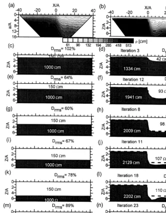
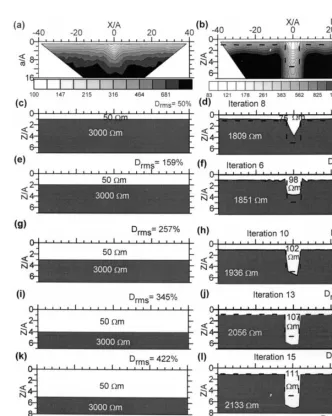
An example of the apparent resistivity pseu-dosection data calculated for a vertical fault model is presented in Fig. 2a. The depth to the top of the fault is 1 A and the fault throw is 4 A. Gaussian noise with an amplitude of 5% was added. There is a steepening of the isoresistivity contours at the position of the fault. The appar-ent resistivity data set was inverted, first with
Ž .
the smooth inversion program RES2DINV and
Ž
next with the block inversion program RESIX
.
IP2DI .
During the smooth inversion of the data, the data rms misfit converged at the end of the fourth iteration. The geometry of the structure is better defined after inversion with respect to the very steep resistivity anomaly at about the
posi-Ž .
tion of the fault Fig. 2b . There are portions of the overburden where the model resistivity is higher than the true value while over the re-maining portion the model resistivities are lower than the true value. The same is true for the model bedrock resistivity. These are due to the smearing effects produced by smooth inversion, especially in the vicinity of zones with an abrupt discontinuity in resistivity.
A two-layer model was employed as the
ini-Ž .
tial starting model for the block inversion. The effect of the depth to the bedrock interface in the initial model on the block inversion was investigated with a structure in which the model parameters include r1Žinitial.s150 Vm and r2Žinitial.s1000 Vm. The HŽinitial. was varied from 1 A to 6 A. It was not possible to obtain a reasonable interpretation in the case with
HŽinitial.s1 A. The best-fit model in this case is shown in Fig. 2d. The pseudosection data
calcu-Ž .
lated from this model Fig. 3a is to a very large extent Aout-of-phaseB with the synthetic ob-served data in Fig. 2a as reflected in the very high data rms misfit. The data misfit section
ŽFig. 3b shows that there are two broad regions.
with negative data misfits, namely, at very shal-low spacings in the upthrown block and at intermediate-to-large spacings in the down-thrown side. On the other hand, there is a near-surface region with positive data misfits to the right-hand side of the fault. Hence, the data misfit is not evenly distributed over the entire section.
An acceptable interpretation, as indicated by a Drms value of about the same level as the amount of Gaussian noise in the data, was produced from the block inversion for larger
Ž .
Fig. 2. a Synthetic pseudosection data calculated for a vertical fault structure, buried by a single overburden unit, with 5%
Ž . Ž . Ž .
Gaussian noise added. b Resistivity image obtained from smooth inversion algorithm. From c to n , the left-hand panel is the starting model used as input for block inversion while the right-hand panel is the inverted model. The dashed line is an outline of the true 2-D model.
and it can be observed that there is an increase in both the overburden and the bedrock resistiv-ity with an increase in the prescribed HŽinitial.. However, if the starting depth is too deep, the inversion results can be unstable. In such in-stances, the depth of the interface of the lower resistive layer in the inverted model begins to undulate, as if a type of ringing occurs. Beard
Ž . Ž .
Ž . Ž .
Fig. 3. The synthetic pseudosection data left-hand panel and the data misfit right-hand panel from some of the best-fit 2-D models from the block inversion of the data in Fig. 2.
3.2. Horst
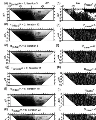
The apparent resistivity pseudosection data calculated from a horst structure in which the depth to the top is 1 A and the throw 4 A is shown in Fig. 4a. The width of the body is 8 A. The overburden resistivity is 100 Vm while that of the bedrock is 2000 Vm. As would be expected, there is a highly resistive structure at the position of the horst. During the inversion of the apparent resistivity pseudosection data with
the smooth inversion algorithm, the data rms misfit converged at the end of the fourth itera-tion and the high resistivity anomaly is correctly
Ž .
positioned Fig. 4b .
The effect of the depth to bedrock interface in the initial two-layer model on the block inversion is shown in Fig. 4c–m, with HŽinitial.
posi-Fig. 4. Inversion of apparent resistivity data over a basement horst structure. The model parameters comprise depth to top
Ž . Ž .
1 A, depth extent 4 A, width 8 A, overburden resistivity 100 Vm and bedrock resistivity 2000 Vm. a Synthetic data. b
Ž . Ž .
Model from smooth inversion. From c to n , the left-hand panel is the starting model used as input for block inversion while the right-hand panel is the inverted model. The dashed line is an outline of the true 2-D model.
tion of the horst structure. The overburden resis-tivity is modelled accurately. The error in the estimate of the bedrock resistivity is very low up till an HŽinitial. of 4 A. The inversion became unstable for larger HŽinitial., and this is reflected in the very high bedrock model resistivity and the markedly undulatory bedrock interface. As with the fault model, variation in the resistivity
contrast in the initial model has only a negligi-ble effect on the inversion results.
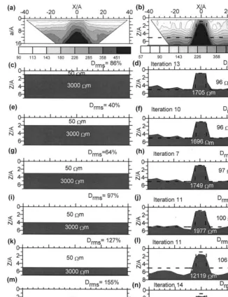
3.3. Graben
shown in Fig. 5a. The width of the structure is 8 A. The overburden unit has a resistivity of 100 V and the bedrock 2000 Vm. As would be expected, there is a low resistivity anomaly at the position of the graben. The model obtained from the smooth inversion of the pseudosection data is presented in Fig. 5b. The presence of a low resistivity anomaly at shallow depths and at the centre of the profile is clearly indicated,
although it is difficult to fix the actual geometry of the bedrock contact.
To investigate the effect of the depth to bedrock interface in the two-layer model used as initial model for the block inversion of the apparent resistivity data, HŽinitial. was varied from 1 A to 6 A. The respective inverted models
ŽFig. 5c–n show that in each case there is a.
low resistivity anomaly at the position of the
Fig. 5. Calculated pseudosection data for a trough structure with a width of 8 A, depth to top 1 A, depth to bottom 5 A,
Ž . Ž . Ž .
graben structure. There is an increase in both the overburden and the bedrock resistivities as
HŽinitial. increases. That the inverted model in Fig. 5n is in error is indicated by the very high data rms misfit. Test with several theoretical examples show that the inversion results are, for all practical purposes, not affected by the layer resistivities in the starting models.
4. Extension to three geoelectric units
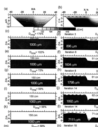
The interpretation procedure described above was extended to 2-D models with two overbur-den units in order to study the influence of equivalence on the result obtained from data inversion. The pseudosection data in Fig. 6a was calculated from a structure in which there is
Fig. 6. The effect of the suppression of a thin surfacial layer on the modelling and inversion of the apparent resistivity data.
Ž .a Synthetic data calculated over a fault model buried under two thin overburden units. b 2-D model obtained from theŽ . Ž . Ž .
Ž .
a thin 0.5 A surfacial relatively conductive layer with a resistivity of 30 Vm. The underly-ing geoelectric unit has a resistivity of 100 Vm. The depth to the top of the fault is 1 A while the throw is 4 A. The bedrock resistivity is 2000 Vm. There is a steepening of the contours in the vicinity of the buried fault. The model from
Ž .
the smooth inversion of the data Fig. 6b shows that the presence of the two overburden units
has reduced the magnitude of the anomaly due to the buried fault.
A two-layer model was employed as the starting model for the block inversion. The depth to the bedrock interface was varied from 1 A to
Ž
6 A. As might be expected, the equivalent or
.
replacement overburden resistivity in the in-verted model is intermediate between the resis-tivities of the two overburden units in the true
Ž .
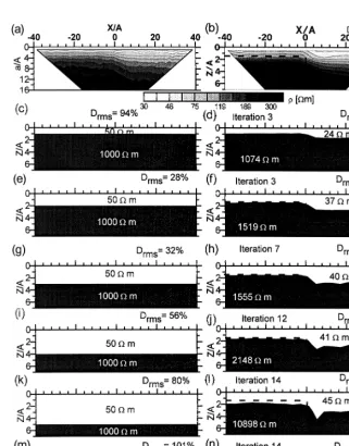
Fig. 7. Inversion of data in the presence of a relatively thick surficial layer. a Synthetic data calculated from the 2-D model.
Ž .b 2-D model obtained from the smooth inversion. From c to n , the left-hand panel is the initial model for blockŽ . Ž .
Ž .
model Fig. 6c to n . The data rms misfit is relatively high for HŽinitial. of 1 A, indicating that the best-fit model in this case isAout-of-phaseB
with the measured data. For larger HŽinitial., up till 4 A, there is a decrease in the error of estimation of the bedrock model resistivity with an increase in HŽinitial.. Although the fault con-tact is correctly located, there is a depth under-estimation in the downthrown block. For larger
HŽinitial., the inversion was unstable, with the data rms misfit and the bedrock model resistiv-ity being relatively high.
If the thickness of the surfacial layer be-comes substantial, it is to be expected that its influence on the pseudosection data, and
conse-quently also, its effect on the inversion results, would become more pronounced. This is illus-trated with a model in which the thickness of the surficial layer is 1 A while its resistivity is 30 Vm. The depth to the top of the fault is 1.5 A while the throw is 3.5 A. The resistivity of the lower unit of the overburden is 100 Vm while that of the basement is 2000 Vm. Both the pseudosection data and the smooth inversion
Ž .
model Fig. 7a and b, respectively indicate that the anomaly is greatly suppressed. There is only a slight steepening isoresistivity contours at depth in the vicinity of the position of the fault. A two-layer model was first employed as the starting model for the block inversion of the
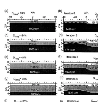
Fig. 8. Re-interpretation of the apparent resistivity data in Fig. 7a employing three geoelectric units. The left-hand panels are the initial models for block inversion while the corresponding inverted models are shown in the right-hand panels. Note that
Ž .
data, with the HŽinitial. varied from 1 A to 6 A. The Drms for the best-fit inverted model in Fig. 7d is relatively high and on account of this, the model is not considered acceptable. Similarly, the bedrock model resistivity for the inverted models in Fig. 7l and n are too high and, for this reason, these models are not considered equiva-lent interpretation of the synthetic observed data. On the other hand, the inversion results for
Ž .
moderate HŽinitial. Fig. 7f, h and j are reason-able interpretations of the data. It may be noted that even for these models, there is an underesti-mation of the depth to the bedrock interface in the downthrown block.
The apparent resistivity data in Fig. 7a were re-interpreted using an initial model comprising three layers in which the resistivities are 50, 200 and 1000 Vm, respectively. The depth to the first interface is 1 A while that to the second interface was varied from 2 A to 6 A. The results obtained after the block inversion are presented in Fig. 8. It can be observed that the resistivity of the first geoelectrical unit is reliably esti-mated. However, the horizontal interface has been converted into a dipping structure as a result of the influence of the underlying faulted block. The model resistivity of the second geo-electric unit varies over a wide range. Similarly, the bedrock model resistivity varies over a wide range.
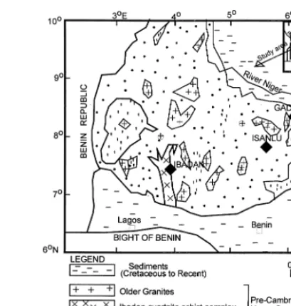
5. Field examples
The interpretation procedure described above has been tested with several case histories from the crystalline basement area of southwestern
Ž .
Nigeria Fig. 9 . The layer resistivities in the initial model for the block inversion have been prescribed based on the range of the measured pseudosection data. The resistivity of the upper layer is of the order of the minimum apparent
Ž
resistivity measured at the shallowest electrode
.
spacing and the bedrock resistivity prescribed
Ž
as the maximum apparent resistivity measured
Fig. 9. Generalised geological map of southwestern Nige-ria showing the study area. A map of NigeNige-ria is presented as inset.
.
at the largest electrode spacing . Representative data sets from one of the sites are presented below.
The field data from Ibadan demonstrate the usefulness of both smooth and block inversion schemes in interpreting data from a low latitude area underlain by crystalline basement rocks. The major rock types in the study area include Older granites, quartzite and quartz-schist, gneisses and undifferentiated metasediments of Pre-Cambrian to Upper Cambrian age. These are often overlain by a thin veneer of regolith materials derived from the chemical weathering of the basement rocks.
are possible from the same set of measured data.
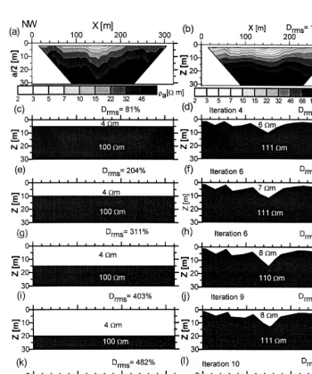
Line 3 is one of the lines measured on the waste dump; the data are between 4 and 90 Vm and there is a low resistivity anomaly between
Ž .
about 120 and 180 m Fig. 10a . The model obtained from the smooth inversion of the field
Ž .
data Fig. 10b indicates a low resistivity
mate-Ž .
rial i.e. the refuse plus leachate overlying a highly resistant bedrock. However, it is difficult to place the refuse-bedrock contact. Conse-quently, as a final step in the interpretation, block inversion of the data was carried out.
An examination of the vertical sets of
appar-Ž
ent resistivities for successive electrode
spac-.
ings beneath each electrode position shows that
Ž . Ž .
Fig. 10. Interpretation of Wenner pseudosection data line 3 from a waste dump site, Ibadan, southwestern Nigeria. a
Ž . Ž . Ž .
there is a very steep vertical gradient, support-ing a strong possibility of a sharp, rather than a
gradational, vertical resistivity change. A two-layer initial model was prescribed in which the
Ž . Ž . Ž .
Fig. 11. Interpretation of Wenner pseudosection data line 5 adjacent to the Ibadan waste dump site. a Measured data. b
Ž . Ž .
resistivity of the upper layer is 4 Vm while that of the bedrock is 100 Vm.
The data rms misfit converged to between 14% and 15% in all the models tested, which is in very good agreement with the result from the smooth inversion. The resistivity of the upper
Ž .
layer representing the refuse shows a slight increase as the thickness of the upper layer in the initial model was increased. This was
ac-companied by an increase in the maximum thickness of the layer from about 10 m in Fig. 10d to about 18 m in Fig. 10l. The ratio of the
Ž
thickness to the resistivity of the layer i.e. its
.
conductance probably remained constant from one inverted model to the other. The bedrock model resistivity varies within a narrow range at between 110 and 114 Vm. These indicate that the resistivities of both geoelectrical units are
Ž . Ž .
Fig. 12. The synthetic pseudosection data left-hand panel and the data misfit right-hand panel from the best-fit 2D models
Ž . Ž . Ž . Ž .
from the block inversion of the data in Fig. 11. a,b HŽinitial.s5 m. c,d HŽinitial.s10 m. e,f HŽinitial.s15 m. g,h
Ž .
well constrained. Similar results were obtained with other initial models tested using different starting resistivities for both the overburden and the bedrock.
The field data presented in Fig. 11a were measured near, but outside, the waste dump site. Here, the apparent resistivities are higher at between 35 and 253 Vm. A high resistivity structure is prominent between 110 and 160 m, this coinciding with the outcrop of the weath-ered basement materials. The model obtained from the smooth inversion of the data is pre-sented in Fig. 11b, with the usual smearing effect noticeable.
In the block inversion, a two-layer model with resistivities of 30 and 300 Vm, respec-tively, was used in modelling the data. The depth to interface was varied between 5 and 25 m. The data rms misfit is within the range of 17% and 19% for HŽinitial. up till 20 m. The overburden model resistivity varies by a factor of about 2 while the bedrock model resistivity varies by a factor of about 1.4. The thickness of the weathering profile in the zone flanking the horst-like structure is expected to range between about 7 and 30 m. The data rms misfit for an
HŽinitial. of 25 m converged to a very high value,
Ž .
indicating that the inverted model Fig. 11l is not an acceptable interpretation of the field data. The synthetic pseudosection data calculated from the best-fit smooth inversion models in Fig. 11, as well as the corresponding data mis-fits, are presented in Fig. 12. It can be observed that the data misfits are low and randomly distributed. However, for Fig. 12j there is an overestimation of the apparent resistivities
Žnegative Di. on the western flank of the high resistivity body. This is due to the very high overburden model resistivity for this model. Moreover, there is an underestimation of the apparent resistivities at the position of the horst structure as expected from the excessive depth to the top of the horst structure.
It should be noted that in this example, the resistivities of the geoelectrical units are reason-ably well constrained. Test with other starting
models show that the resistivity contrast in the initial model has only a negligible effect on the inversion results.
6. Discussion and conclusions
In this paper, a comparison has been made between inversion results with smooth and block inversion schemes. It should be stressed that all
Ž .
inversion methods make assumption s about the resistivity distribution of the subsurface which are implemented in the form of con-strains. The accuracy of the results depends to a large extent on whether or not the actual subsur-face agrees with these assumptions. The smoothness-constrained method assumes the subsurface resistivity varies in a smooth manner and it attempts to minimise the changes in resistivity in a least-squares sense. In cases where the subsurface resistivity varies in a smooth manner, for example chemical pollution
Ž .
plumes Barker, 1996 , this approach will per-form very well. On the other hand, the block inversion method assumes that the subsurface consists of a few homogeneous regions with a sharp interface between them. Such an inversion scheme would be the logical choice where the subsurface comprises units with sharp bound-aries in order to determine both layer boundary
Ž
locations and layer resistivities accurately Ellis
.
and Oldenburg, 1994a; Smith et al., 1999 . The synthetic examples chosen for this paper agree exactly with the assumptions made by the block
Ž .
resistive layer in the inverted model begins to undulate, as if a type of ringing occurs. Beard
Ž . Ž .
and Morgan 1991 and Oldenburg and Li 1999 have also described such unusual inversion ef-fects at the edges of 2-D structures. These weaknesses can be easily overcome by a com-bined use of a cell-based inversion method and the block inversion method. The cell-based in-version will at least give a rough idea of the bedrock depth which will prevent the starting depth in the block inversion to be too shallow or too deep, particularly with field data. The cell-based inversion model can also warn the user if the subsurface is more complex than the two regions model. The different inversion methods described can be viewed as complementary tools the interpreter can employ to obtain the most consistent and reasonable results for a given data set.
Acknowledgements
This work was carried out in the Department of Applied Geophysics, Technical University, Berlin. The authors are grateful to the Alexan-der von Humboldt Foundation, Bonn, who funded AIO as research fellow. Les P. Beard, Editor-in-Chief N.B. Christensen and an anony-mous reviewer are thanked for their suggestions which greatly improved the paper.
References
Barker, R.D., 1992. A simple algorithm for electrical
Ž .
imaging of the subsurface. First Break 10 2 , 53–62. Barker, R.D., 1996. Application of electrical tomography
in groundwater contamination studies. EAGE 58th Conference and Technical Exhibition Extended Ab-stracts. p. P082.
Beard, L.P., Morgan, F.D., 1991. Assessment of 2-D resistivity structures using 1-D inversion. Geophysics 56, 874–883.
Carruthers, R.M., Smith, I.F., 1992. The use of ground electrical survey methods for siting water-supply bore-holes in shallow crystalline basement terrains. In:
Ž .
Wright, E.P., Burgess, W.G. Eds. , Hydrogeology of
Crystalline Basement Aquifers in Africa. Geological Society Special Publication No. 66, pp. 203–220. Dahlin, T., Loke, M.H., 1998. Resolution of 2D Wenner
resistivity imaging as assessed by numerical modelling. J. Appl. Geophys. 38, 237–249.
DeGroot-Hedlin, C., Constable, C., 1990. Occam’s inver-sion to generate smooth two-dimeninver-sional models from magnetotelluric data. Geophysics 55, 1613–1624. Ellis, R.G., Oldenburg, D.W., 1994a. Applied geophysical
inversion. Geophys. J. Int. 116, 5–11.
Ellis, R.G., Oldenburg, D.W., 1994b. The pole–pole 3D DC resistivity inverse problem: a conjugate-gradient approach. Geophys. J. Int. 119, 187–194.
Griffiths, D.H., Barker, R.D., 1993. Two-dimensional re-sistivity imaging and modelling in areas of complex geology. J. Appl. Geophys. 29, 211–226.
Hazell, J.R.T., Cratchley, C.R., Jones, C.R.C., 1992. The hydrogeology of crystalline aquifers in northern Nigeria and geophysical techniques used in their exploration.
Ž .
In: Wright, E.P., Burgess, W.G. Eds. , Hydrogeology of Crystalline Basement Aquifers in Africa. Geological Society Special Publication No. 66, pp. 155–182. Inman, J.R., 1985. Resistivity inversion with ridge
regres-sion. Geophysics 50, 2112–2131.
Interpex, 1996. RESIX IP2DI v3, Resistivity and induced polarization data interpretation software. Interpex, Golden, Colorado.
Koefoed, O., 1979. Geosounding Principles: 1. Resistivity Sounding Measurements. Elsevier, Amsterdam, 276 pp. Loke, M.H., Barker, R.D., 1995. Improvements to the Zohdy method for the inversion of resistivity sounding
Ž .
and pseudosection data. Comput. Geosci. 21 2 , 321– 332.
Loke, M.H., Barker, R.D., 1996. Rapid least-squares inver-sion of apparent resistivity pseudosections by a quasi-Newton method. Geophys. Prospect. 44, 131–152. Marquardt, D.W., 1963. An algorithm for least-squares
estimation of nonlinear parameters. J. Soc. Ind. Appl. Math. 11, 431–441.
Muiuane, E.A., Pedersen, L.B., 1999. Automatic 1D inter-pretation of DC resistivity sounding data. J. Appl. Geophys. 42, 35–45.
Oldenburg, D.W., Li, Y., 1999. Estimating depth of inves-tigation in dc resistivity and IP surveys. Geophysics 64, 403–416.
Pelton, W.H., Rijo, L., Swift, C.M., 1978. Inversion of two-dimensional resistivity and induced-polarization data. Geophysics 43, 788–803.
Petrick, W.R., Pelton, W.H., Ward, S.H., 1977. Ridge regression applied to crustal resistivity sounding data from South Africa. Geophysics 42, 995–1005. Rijo, L., 1977. Electromagnetic modeling by the finite
least-squares inversion schemes for studying equiva-lence in one-dimensional resistivity interpretation. Geo-physics 57, 1282–1293.
Smith, T., Hoversten, M., Gasperikova, E., Morrison, F., 1999. Sharp boundary inversion of 2D magnetotelluric data. Geophys. Prospect. 47, 469–486.
Zohdy, A.A.R., 1974. Use of Dar Zarrouk curves in the interpretation of vertical electrical sounding data. US Geol. Surv. Bull. 1313-D, 41.