Homogeneous risk models with equalized claim amounts
q
F. De Vylder
a, M. Goovaerts
a,b,∗aUniversiteit van Amsterdam, Amsterdam, Netherlands
bKatholieke Universiteit Leuven, CRIR, Huid Eygen Heerd, Minderbroederstraat 5, 3000 Leuven, Belgium
Received 1 June 1998; received in revised form 1 September 1999; accepted 24 November 1999
Abstract
We consider an homogeneous risk model on a fixed bounded time interval [0, t] and we denote by Nt the number of
claims in that interval. The claim amounts areX1, X2, . . . , XNt. The homogeneous model is an extension of the classical
actuarial risk model with Nt not necessarily Poisson distributed. In the model with equalized claim amounts, each amount
Xk is replaced withXk∼ = (X1+ · · · +XNt)/Nt. Let9(t, u) be the ruin probability before t in the homogenous model,
corresponding to the initial risk reserve u≥0 and let9∼(t, u) be the corresponding ruin probability evaluated in the
associ-ated model with equalized claim amounts. The essence of the classical Prabhu formula is that9(t, 0)=9∼(t, 0). By rather systematic numerical investigations in the classical risk model, we verify that9∼(t, u)≤9(t, u) for any value of u≥0 and
that9∼(t, u) is an excellent approximation of9(t, u). Then these conclusions must be valid in any homogeneous model and this is an interesting observation because9∼(t, u) can be calculated numerically, whereas no algorithms are yet
avail-able for the numerical evaluation of9(t, u) in general homogeneous risk models. © 2000 Elsevier Science B.V. All rights reserved.
Keywords: Risk model; Homogeneous risk model; Ruin probability; Prabhu’s formula
1. Homogeneous risk model on a bounded time interval [0,ttt]
Nt is the number of claims in [0, t]. The claim instants process (T1, T2, . . . , TNt) is any homogeneous point process on the fixed interval [0, t]. Its distribution is completely specified by the probabilities P(Nt=n)≥0 (n=0, 1,
2,. . .) such that6n≥0P(Nt=n)=1. The latter probabilities may be any numbers satisfying the indicated relations
(see Appendix of De Vylder and Goovaerts (1999)). The claim amounts areX1, X2, . . . , XNt. It is assumed that
X1, X2,. . . are i.i.d. random variables with distribution function F concentrated on [0,∞) and that these amounts
are independent from the claim instants. The risk reserve process is Rτ=u+cτ−Sτ(0≤τ≤t), where u≥0 is the initial
risk reserve, c>0 the premium income rate and Sτ the total claim amount in [0,τ], i.e.Sτ =X1+ · · · +XNt, where
Nτ is the number of claims in [0,τ]. Of course, Sτ=0, if Nτ=0.
q
Presented at the Second International IME Congress, University of Lausanne, Switzerland, July 1998. ∗Corresponding author. Tel.:+32-16-323-746; fax:+32-16-323-740.
E-mail address: [email protected] (M. Goovaerts)
We denote by U(t, u) the probability of nonruin before t corresponding to the initial risk reserve u≥0, and by
Un(t, u) the corresponding conditional probability of nonruin for fixed Nt=n. Then
U (t, u)=X
n≥0
P (Nt=n)Un(t, u). (1)
The homogeneous model with fixed Nt=n is defined by the probabilities P(Nt=n)=1 and P(Nt=m)=0 (m6=n).
Then Un(t, u) is the (nonconditional) probability of ruin in the homogeneous model with fixed Nt=n. In the
homogeneous model with fixed Nt=n, the claim instants areT1< T2<· · ·< Tnand the random vector (T1,. . ., Tn) has a constant density on the subsetWtn = {(t1, . . . , tn)|0 < t1 < t2 <· · ·< tn < t}of Rn. The Lebesgue
volume of Wtnis tn/n!. Hence the density of (T1,. . ., Tn) equals n!/tnon Wtn. Then, by the foregoing assumptions,
the distribution of the random vector (T1,. . ., Tn, X1,. . ., Xn) is completely specified in the homogeneous model
with fixed Nt=n.
2. Nonruin probability before timetttin the homogeneous model
Letτ, y1, y2,. . . be any numbers. The numbers z0=1, z1, z2,. . . are defined recursively as follows:
The first numbers zkare
z0=1, z1= −y1, z2= −
Ik+1(y1, . . . ,yk+1,τ )=
We recall that X1, X2,. . . are the i.i.d. claim amounts with distribution function F and that u≥0 is the initial risk
reserve. We define
We notice that this is relation (2) with capital letters everywhere. The first random variables Zkare
Z0=1, Z1= −Y1= −(X1−u)+,
the proof, are finite. Later in this paper, the lemma is only used with the particular function
ϕ(X1, . . . ,Xn)=1(X1+ · · · +Xn≤u+ct),
where 1(.) is the indicator function of a proposition. Then all expectations are integrals with respect to dF(x1)· · ·dF(xn)
of a bounded function on a bounded integration domain of Rn, and they are finite indeed.
and
E[Zkϕ(X1, . . . ,Xn)]=0 (k=2,3, . . . ,n) (9)
if all involved expectations are finite.
Proof. The proof results from the adequate use of the following remark. Let us consider an expectation such as
E[f(X1,. . ., Xk)ϕ(X1,. . ., Xn)], where k≤n. By the i.i.d. assumption on X1, X2,. . ., we may replace X1,. . ., Xn
We now consider (9) for k=3. Then the expectation is the sum of the two terms
E
A general proof by induction is direct. It is based on (7). In the last member of that relation, the first two terms
must be treated jointly; all other terms can be treated separately.
In Theorem 1, F∗nis of course the distribution function of the total claim amountX1+· · ·+Xnin the homogeneous
model with fixed Nt=n. The function Inis the n-tuple integral defined by (3). Of course U0(t, u)=1 because ruin
cannot occur if there are no claims.
In the general homogeneous model on [0, t], we denote by Ft the distribution function of the total claim amount St=X1+X2+ · · · +XNt in [0, t].
a. In the homogeneous model with fixed Nt=n,
b. In the homogeneous model with fixed Nt=n and u=0,
c. (Prabhu’s formula) In the general homogeneous model on [0, t] with u=0,
U (t ,0)=
probability Un(t, u) equals
Un(t ,u)=n!t−n
These relations are equivalent to the relations
x1≥0, . . . ,xn≥0, x1+ · · · +xn≤u+ct , (16)
b. Let us now assume that u=0. By Lemmas 1 and 2, In(Y1,. . ., Yn, ct) can be replaced with (ct)n
n! −
(Yn/n)(ct)n−1 (n−1)! =(ct)
n(n!)−1
1−Yn
ct
in (13). This proves the first relation (14). The second relation (14) is obvious. Then the last relation (14) results from an integration by parts.
c. (15) results from (1), (12) and (14).
General expectations such as E[ϕ(X1,. . ., Xn)] are almost impossible to evaluate numerically, fastly and precisely
enough, if n is large. In particular, (13) is not useful for the practical evaluation of Un(t, u).
On the contrary, expectations such asE[ϕ(X1+ · · · +Xn)] can be calculated. Indeed, they are reduced to single
integrals
E[ϕ(X1+ · · · +Xn)]= Z
I
ϕ(y)dF∗n(y).
In practice I is a bounded interval and F the discretized, i.e. F is hold back as a long vector in the computer program. Then F∗ncan be calculated iteratively and only two successive long vectors F∗kand F∗(k+1)(k=1,2,. . .,
n) must be stored simultaneously in the process at each stage.
If the discretized F hasνcomponents, then the direct calculation of
E[ϕ(X1, . . . ,Xn)]= Z
· · ·
Z
D
ϕ(x1, . . . ,xn)dF (x1)· · ·dF (xn)
may need the evaluation ofνnterms, to be summed up. In the case of U
n(t, u) the evaluation ofϕ(x1,. . ., xn) goes
via relations such as (4). All this must be done for values n=0, 1, 2,. . ., n0and then U(t, u) should result from
(1). In some casesνand n0may be pretty large, sayν=1000 and n0=100. Clearly this rudimentary procedure is
hopeless, even with the fastest computers available today.
3. Homogeneous model with equalized claim amounts
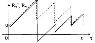
We now start from an homogeneous model with time interval [0, t], called the initial model, and we replace each claim amount Xkwith the average amountXk∼=(X1+ · · · +XNt)/Nt. This model with equalized claim amounts is also called the associated model. The claims instants Tk(k=1, 2,. . ., Nt) are the same in both models:Tk∼=Tk. The
superscript∼is used systematically for the components of the associated model with equalized claim amounts. We notice that the risk reserveRτ∼(0≤τ ≤t )cannot be determined from observations during time interval [0,τ]. The
complete trajectory Rs(0≤s≤t) is necessary in order to fixRτ∼. The distribution of the trajectoriesRτ∼(0≤τ ≤t )
results from the distribution of the trajectories Rτ(0≤t≤t). Hence, the associated model is clearly defined. In Figs.
1–4, we represent sample functions of the processes Rτ (full lines) andRτ∼(stippled lines). All four following
cases a, b, c and d can occur.
a. No ruin in the initial model, no ruin in the associated model (Fig. 1), b. Ruin in the initial model, ruin in the associated model (Fig. 2), c. No ruin in the initial model, ruin in the associated model (Fig. 3), d. Ruin in the initial model, no ruin in the associated model (Fig. 4).
Due to compensations between occurrences of these cases, the following question is relevant: is U∼(t, u) close to
U(t, u)? The most surprising answer is that in case of an initial risk reserve u=0, the compensation is perfect: U∼(t, 0)=U(t, 0) (Theorem 2b). This throws a new light on Prabhu’s formula. The numerical investigations of Section 5
Fig. 1. No ruin in initial model. No ruin in associated model.
Fig. 2. Ruin in initial model. Ruin in associated model.
Fig. 3. No ruin in initial model. Ruin in associated model.
Table 1
Uniform F,η=0.05, t=1
u 9 9∼
0 0.527 0.527
1 0.0925 0.0920
2 0.00827 0.00832
3 0.00049 0.00050
4 0.00002 0.00002
Table 2
Uniform F,η=0.05, t=5
u 9 9∼
0 0.777 0.777
1 0.346 0.320
2 0.113 0.105
3 0.0297 0.0281
4 0.00646 0.00622
5 0.00119 0.00117
6 0.00019 0.00019
Table 3
Uniform F,η=0.05, t=10
u 9 9∼
0 0.835 0.835
1 0.473 0.433
2 0.221 0.199
3 0.0900 0.0814
4 0.0321 0.0294
5 0.0101 0.00940
6 0.00284 0.00269
7 0.00072 0.00070
8 0.00016 0.00016
Table 4
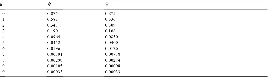
Uniform F,η=0.05, t=20
u 9 9∼
0 0.875 0.875
1 0.583 0.536
2 0.347 0.309
3 0.190 0.168
4 0.0964 0.0850
5 0.0452 0.0400
6 0.0196 0.0176
7 0.00791 0.00718
8 0.00298 0.00274
9 0.00105 0.00098
Table 5
Uniform F,η=0.25, t=1
u 9 9∼
0 0.505 0.505
1 0.0822 0.0810
2 0.00734 0.00685
3 0.00038 0.00040
4 0.00002 0.00002
Table 6
Uniform F,η=0.25, t=5
u 9 9∼
0 0.710 0.710
1 0.265 0.239
2 0.0742 0.0670
3 0.0172 0.0158
4 0.00335 0.00316
5 0.00056 0.00054
6 0.00008 0.00008
Table 7
Uniform F,η=0.25, t=10
u 9 9∼
0 0.753 0.753
1 0.343 0.300
2 0.130 0.111
3 0.0441 0.0379
4 0.0134 0.0117
5 0.00368 0.00328
6 0.00091 0.00083
7 0.00021 0.00019
8 0.00004 0.00004
Table 8
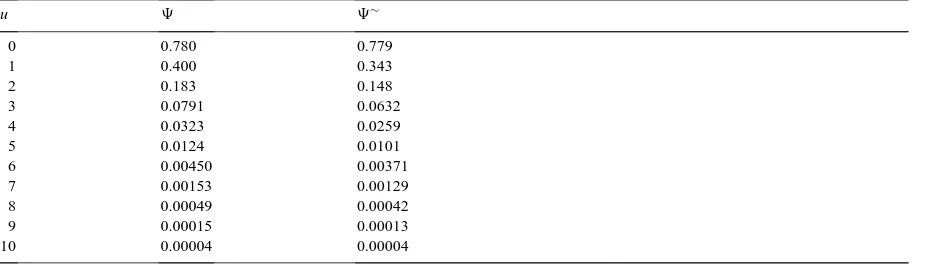
Uniform F,η=0.25, t=20
u 9 9∼
0 0.780 0.779
1 0.400 0.343
2 0.183 0.148
3 0.0791 0.0632
4 0.0323 0.0259
5 0.0124 0.0101
6 0.00450 0.00371
7 0.00153 0.00129
8 0.00049 0.00042
9 0.00015 0.00013
Table 9
Exponential,η=0.05, t=1
u 9 9∼
0 0.470 0.470
2 0.122 0.120
4 0.0293 0.0290
6 0.00671 0.00667
8 0.00146 0.00147
10 0.00031 0.00031
Table 10
Exponential,η=0.05, t=5
u 9 9∼
0 0.735 0.735
2 0.370 0.325
4 0.168 0.146
6 0.0702 0.0618
8 0.0274 0.0245
10 0.0100 0.00915
12 0.00349 0.00325
14 0.00117 0.00111
16 0.00038 0.00036
Table 11
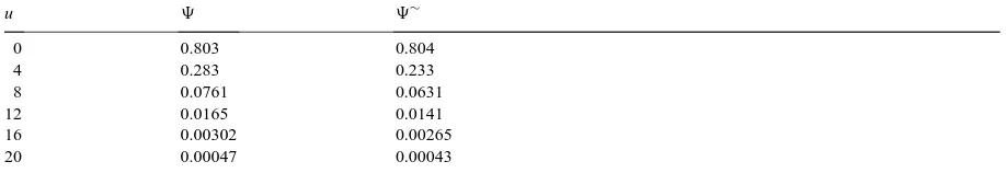
Exponential,η=0.05, t=10
u 9 9∼
0 0.803 0.804
4 0.283 0.233
8 0.0761 0.0631
12 0.0165 0.0141
16 0.00302 0.00265
20 0.00047 0.00043
Table 12
Exponential,η=0.05, t=20
u 9 9∼
0 0.852 0.853
4 0.408 0.328
8 0.164 0.129
12 0.0565 0.0447
16 0.0168 0.0136
20 0.00436 0.00368
24 0.00103 0.00089
Table 13
numerically in that case only (as far as we know). By arguments of De Vylder and Goovaerts (1999, Section 6) the validity of results in the classical model can often be extended to any homogeneous model.
By the discussion at the end of foregoing Section 2 and by next formula (19) combined with the (∼)-version of (1), the nonruin probability U∼(t, u) can be calculated in any homogeneous model.
4. Nonruin probability beforetttin case of equalized claim amounts
Theorem 2.
a. In the homogeneous risk model with fixed Nt=n and equalized claim amounts,
Un∼(t ,u)=n!(ct)−nE
b. (Interpretation of Prabhu’s formula). In the general homogenous model on[0, t] and its associated model with
equalized claim amounts,
a. The second relation (19) is obvious because F∗nis the distribution function of Sn. For the first relation (19) it is
enough to repeat the proof of Theorem 1a. Nowx1+· · ·+xkmust everywhere be replaced withk(x1+· · ·+xn)/n
Table 15
Exponential,η=0.25, t=10
u 9 9∼
0 0.729 0.729
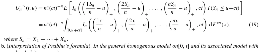
4 0.204 0.153
8 0.0463 0.0351
12 0.00886 0.00698
16 0.00148 0.00120
20 0.00022 0.00018
Table 16
Exponential,η=0.25, t=20
u 9 9∼
0 0.764 0.765
4 0.272 0.187
8 0.0859 0.0568
12 0.0241 0.0163
16 0.00603 0.00427
20 0.00137 0.00101
24 0.00028 0.00022
28 0.00005 0.00004
Table 17
Pareto,η=0.05, t=1
u 9 9∼
0 0.531 0.531
10 0.0124 0.0124
20 0.00275 0.00277
30 0.00119 0.00118
40 0.00066 0.00065
b. It is sufficient to consider the model with fixed Nt=n and equalized claim amounts and to prove that
Un∼(t ,0)= Z
[0,ct] h
1− x
ct i
dF∗n(x) (21)
because then (20) results from (15), (1) and the (∼)-version of (1). Now (kx/(n−u))+=kx/n because u=0. Then, by (5),
In 1x
n , 2x
n, . . . ,
nx
n,ct
=(ct)
n
n! −
(x/n)(ct)n−1 (n−1)!
and then (21) results from (19).
We denote by9(t, u)=1−U(t, u) and9∼(t, u)=1−U∼(t, u) the ruin probabilities before time t corresponding to the initial risk reserve u≥0. Sometimes different values of the premium income rate c are considered simultaneously. Then we write more explicitly9(t, u, c) and9∼(t, u, c).
4.1. Conjecture
In any homogeneous risk model with time interval [0, t] and its associated model with equalized claim amounts,
Table 18
Pareto,η=0.05, t=5
u 9 9∼
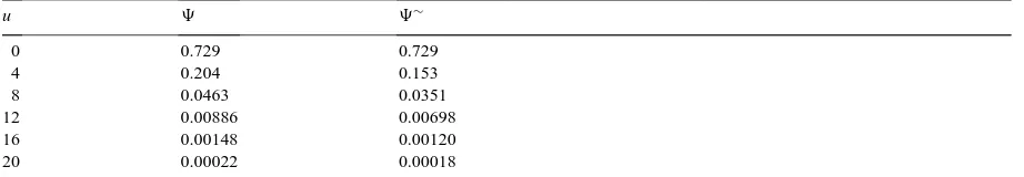
0 0.745 0.745
10 0.0798 0.0742
20 0.0175 0.0166
30 0.00690 0.00662
40 0.00364 0.00352
50 0.00224 0.00219
60 0.00152 0.00149
70 0.00110 0.00108
80 0.00083 0.00082
Table 19
Pareto,η=0.05, t=10
u 9 9∼
0 0.802 0.803
20 0.0409 0.0365
40 0.00802 0.00741
60 0.00323 0.00305
80 0.00173 0.00166
100 0.00108 0.00104
120 0.00074 0.00072
Table 20
Pareto,η=0.05, t=20
u 9 9∼
0 0.845 0.847
20 0.0908 0.0758
40 0.0185 0.0161
60 0.00707 0.00634
80 0.00369 0.00338
100 0.00226 0.00211
120 0.00153 0.00144
140 0.00110 0.00106
160 0.00084 0.00080
Table 21
Pareto,η=0.25, t=1
u 9 9∼
0 0.496 0.496
10 0.0117 0.0117
20 0.00270 0.00270
30 0.00117 0.00116
Table 22
Pareto,η=0.25, t=5
u 9 9∼
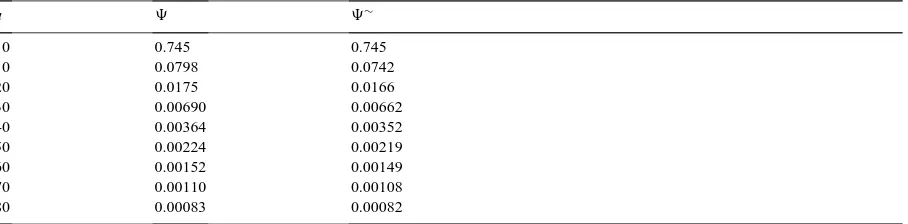
0 0.674 0.675
10 0.0631 0.0562
20 0.0151 0.0138
30 0.00625 0.00587
40 0.00338 0.00322
50 0.00212 0.00204
60 0.00146 0.00141
70 0.00106 0.00103
80 0.00081 0.00079
Table 23
Pareto,η=0.25, t=10
u 9 9∼
0 0.720 0.721
20 0.0307 0.0256
40 0.00694 0.00612
60 0.00294 0.00269
80 0.00162 0.00151
100 0.00102 0.00097
120 0.00071 0.00068
Table 24
Pareto,η=0.25, t=20
u 9 9∼
0 0.751 0.753
20 0.0566 0.0415
40 0.0138 0.0109
60 0.00585 0.00490
80 0.00322 0.00279
100 0.00204 0.00181
120 0.00140 0.00127
140 0.00103 0.00094
160 0.00079 0.00073
Table 25
Uniform,η=0.25, t=10
u 9sqrt 9∼
0 0.743 0.743
1 0.366 0.308
2 0.126 0.128
3 0.0637 0.0561
4 0.0292 0.0227
5 0.0108 0.00735
6 0.00296 0.00170
Table 26
Exponential,η=0.25, t=10
u 9sqrt 9∼
0 0.719 0.719
2 0.369 0.325
4 0.167 0.166
6 0.0953 0.0864
8 0.0522 0.0444
10 0.0273 0.0221
12 0.0136 0.0105
14 0.00639 0.00478
16 0.00285 0.00206
18 0.00121 0.00085
20 0.00048 0.00033
Table 27
Pareto,η=0.25, t=10
u 9sqrt 9∼
0 0.711 0.711
10 0.109 0.103
20 0.0332 0.0292
30 0.0135 0.0121
40 0.00710 0.00652
50 0.00436 0.00407
60 0.00295 0.00279
70 0.00214 0.00204
80 0.00162 0.00155
90 0.00127 0.00122
100 0.00102 0.00099
110 0.00084 0.00082
This Conjecture is based on the numerical study of Section 6. By (1) and its (∼)-version, it is equivalent to the proposition:9n∼(t, u)≤9n(t, u)for all n=1, 2,. . .. Of course,91∼(t, u)=91(t, u). The proof of92∼(t, u)≤
92(t, u)is rather direct by (13) and (19) and by the arguments of the proof of Lemma 2. The proof of the general
case is still missing.
5. Numerical illustrations
5.1. Parameters
In the classical model, we display c as c=λµ(1+η), whereηis the security loading,µthe first moment of the claimsize distribution andλthe parameter of the Poisson claim instants process. We takeλ=1 and we consider the values 1, 5, 10, 20 of t. We consider the valuesη=0.05 andη=0.25 of the security loading. For the initial risk reserve u we adopt values 0, k, 2k,. . ., mk depending on the other parameters. The integers k and m are fixed in such a way that m≤10 and that the ruin probability corresponding to the last value km is less than 1/1000.
5.2. Claimsize distributions F
Atomic concentrated at 1 F(x)=1 (0≤x≤1), F(x)=1 (x>1). Thenµ=1.
Table 28
Atomic F,η=0.05, t=5
u 9 9∼
0 0.804 0.803
2 0.301 0.300
4 0.0724 0.0723
6 0.0125 0.0124
8 0.00161 0.00160
10 0.00016 0.00015
Exponential F(x)=1−e−x (x≥0). Thenµ=1.
Pareto F(x)=(1−x−2)1 (x≥1) (x≥0). Thenµ=2.
Distribution of Nt. In the classical model, the distribution of Nt is the exponential with parameterλt. We consider
one nonclassical case. It is the homogeneous model on [0, t], t=10, with
P (Nt =n)=cexp[−(10−n)1/2] (n=0,1,2, . . . ,20), P (Nt =n)=0 (n >20),
where c results from the norm relation6n≥0P(Nt=n)=1, i.e. c=0.271940. Then ENt=10 for reasons of symmetry.
We takeλ=ENt/t=1. The nonclassical case is treated with various claimsize distributions.
5.3. Numerical calculations
The claimsize distributions are truncated and finely discretized, with conservation of first momentµ, as explained in De Vylder (1996, p. 268−271). The exact ruin probabilities in the classical model, 9(t, u)=1−U(t, u), are
calculated as explained in the same book p. 257−268, with claimsize distribution and security loading adaptations. In the associated model, the ruin probabilities are evaluated via (19) and the (∼)-version of (1). In the nonclassical case, we cannot evaluate9(t, u) numerically. Instead, we then consider the approximation9sqrt(t, u) defined by De
Vylder and Goovaerts (1999, Section 6).
5.4. Numerical anomalies
By (20),
9(t,0)=9∼(t,0),
This relation and the conjecture of Section 4 are very slightly contradicted at a few places in following tables, because the numerical values include discretization, truncation and decimalization errors and because 9∼(t, u) and9(t, u) are obtained by completely different algorithms. For instance, in Table 28 below, we should have9(t,
u)=9∼(t, u) for all values of u, because the model with equalized claims amounts is the same as the initial model when F is atomic. We have verified that with finer discretizations than those used in the tables, the contradictions disappear. Unfortunately, the finer discretizations cannot be used systematically because then the computing time would be excessive (on our 1995 P.C)
Each of Tables 1–27 (classical cases,l=1) corresponds to the table with the same number in De Vylder and
Goovaerts (1999). The atomic claimsize distribution F (Table 28), is not considered in the latter paper.
References
De Vylder, F.E., 1996. Advanced Risk Theory. A Self-Contained Introduction. Editions de l’Université de Bruxelles, Swiss Association of Actuaries.