BUILDING CHANGE DETECTION FROM LIDAR POINT CLOUD DATA BASED ON
CONNECTED COMPONENT ANALYSIS
Mohammad Awrangjeba,∗, Clive S. Fraserband Guojun Lua
a
School of Engineering and Information Technology, Federation University - Australia Churchill Vic 3842 Australia - (Mohammad.Awrangjeb, Guojun.Lu)@federation.edu.au b
CRC for Spatial Information, Dept. of Infrastructure Engineering, University of Melbourne Parkville Vic 3010, Australia - [email protected]
WG III/4
KEY WORDS:Building detection, change detection, map update, automation, LIDAR, point cloud data
ABSTRACT:
Building data are one of the important data types in a topographic database. Building change detection after a period of time is necessary for many applications, such as identification of informal settlements. Based on the detected changes, the database has to be updated to ensure its usefulness. This paper proposes an improved building detection technique, which is a prerequisite for many building change detection techniques. The improved technique examines the gap between neighbouring buildings in the building mask in order to avoid under segmentation errors. Then, a new building change detection technique from LIDAR point cloud data is proposed. Buildings which are totally new or demolished are directly added to the change detection output. However, for demolished or extended building parts, a connected component analysis algorithm is applied and for each connected component its area, width and height are estimated in order to ascertain if it can be considered as a demolished or new building part. Finally, a graphical user interface (GUI) has been developed to update detected changes to the existing building map. Experimental results show that the improved building detection technique can offer not only higher performance in terms of completeness and correctness, but also a lower number of under-segmentation errors as compared to its original counterpart. The proposed change detection technique produces no omission errors and thus it can be exploited for enhanced automated building information updating within a topographic database. Using the developed GUI, the user can quickly examine each suggested change and indicate his/her decision with a minimum number of mouse clicks.
1. INTRODUCTION
Automation in building change detection is a key issue in the up-dating of building information in a topographic database. There is increased need for map revision, without large increases in cost, in order to keep the mapping current, especially in those areas which are subject to dynamic change due to new construction and reconstruction of urban features such as building and roads. An updated topographic map along with the required building and road information can be used for a multitude of purposes, including urban planning, identification of informal settlements, telecommunication planning and analysis of noise and air pollu-tion. The availability of high resolution aerial imagery and LI-DAR (Light Detection And Ranging) point cloud data has facili-tated increased automation within the updating process.
Automatic building change detection from remote sensing data mainly falls into two categories (Grigillo et al., 2011). Firstly, in thedirectapproach, data acquired from one type of sensor at two different dates are directly compared to detect changes. Sec-ondly, in theindirectapproach, the building information is first detected from a new data set and then compared to that in the ex-isting map. For instance, while (Murakami et al., 1999) detected building changes by simply subtracting DSMs (Digital Surface Models) collected on different dates, (Vosselman et al., 2005) first segmented the normalised DSM in order to detect buildings and then compared them to buildings in the map.
The result of automatic building change detection is subsequently used for updating the existing building map. Since the result may not be 100% correct, some manual work is still required while
∗Corresponding author.
updating the database. (Murakami et al., 1999) suggested that omission error (e.g. missing new and/or demolished buildings and/or building parts) in automatic change detection has to be avoided completely in order to keep human involvement to a min-imum. This is because in the worst case scenario a possibility of omission error would require a manual inspection of the entire original data. Thus, as long as no omission errors are included in the result, removal of commission errors (e.g., false identification of new and/or demolished buildings and/or building parts) can be made in a straightforward manner by focusing expensive manual inspection only on detected changes, which can then reduce the time required to investigate the whole area of interest.
In 2009, under a project of the European Spatial Data Research organisation, (Champion et al., 2009) compared four building change detection techniques and stated that only the method of (Rottensteiner, 2007) had achieved a relatively acceptable result. Nevertheless, the best change detection technique in their study was still unsuccessful in reliable detection of small buildings. So, there is significant scope for investigation of new automatic build-ing change detection approaches.
map database is actually updated. The GUI can be facilitated with an orhtophoto of the study area.
2. RELATED WORK
For both building detection and change detection, there are three categories of technique, based on the input data: image only (Ioannidis et al., 2009, Champion et al., 2010), LIDAR only (Vos-selman et al., 2005) and the combination of image and LIDAR (Rottensteiner, 2007). The comprehensive comparative study of (Champion et al., 2009) on building change detection techniques showed that LIDAR-based techniques offer high economic effec-tiveness. Thus, this paper concentrates on techniques that use at least LIDAR data.
Amongst reported building detection approaches, (Rottensteiner, 2007) employed a classification using the Dempster-Shafer the-ory of data fusion to detect buildings from LIDAR derived DSMs and multi-spectral imagery. For building detection from LIDAR point cloud data alone, (Zhang et al., 2006) first separated the non-ground points from the ground points using a progressive morphological filter. The buildings were then separated from trees using non-ground points by applying a region-growing algo-rithm based on a plane-fitting technique. (Awrangjeb and Fraser, 2014b) simply applied a height threshold to separate the ground and non-ground points. A region growing technique was then ap-plied to grow planes on the stable seed points. A set of rules were applied to remove planes constructed on trees. Finally, neigh-bouring planes were combined to form individual building bound-aries. Reviews of other building detection techniques can be found in (Zhang et al., 2006, Awrangjeb and Fraser, 2014b).
In regard to building change detection, (Zong et al., 2013) pro-posed a direct change detection technique by fusing high-resolution aerial imagery with LIDAR data through a hierarchical machine learning framework. After initial change detection, a post pro-cessing step based on homogeneity and shadow information from the aerial imagery, along with size and shape information of build-ings, were applied to refine the detected changes. Promising re-sults were obtained in eight small test areas. (Murakami et al., 1999) subtracted one of the LIDAR DSMs from three others ac-quired on four different dates. The difference images were then rectified using a straightforward shrinking and expansion filter that reduced the commission errors. The parameter of the filter was set based on prior knowledge about the horizontal error in the input LIDAR data. The authors reported no omission error for the test scene, but they did not provide any statistics on the other types of measurements.
Among the indirect approaches to building change detection, (Matikainen et al., 2010) used a set of thresholds to determine building changes and showed that the change detection step is di-rectly affected by the preceding building detection step, particu-larly when buildings have been missed due to low height and tree coverage. Thus, a set of correction rules based on the existing building map was proposed and the method was tested on a large area. High accuracy was achieved (completeness and correctness were around 85%) for buildings larger than 60 m2, however the method failed to detect changes for small buildings.
(Grigillo et al., 2011) used the exclusive-OR operator between the existing building map and the newly detected buildings to obtain a mask of building change. A set of overlap thresholds (similar to (Matikainen et al., 2010)) to identifydemolished,new,extended
anddiscovered old(unchanged) buildings was then applied and a per-buildingcompletenessandcorrectnessof 93.5% and 78.4%, respectively, was achieved. (Rottensteiner, 2007) compared two
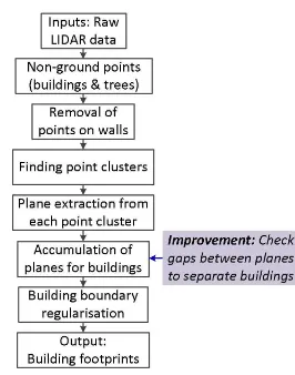
Figure 1: The proposed building detection technique.
label images (from the existing map and automatic building de-tection) to decide building changes (confirmed,changed,newand
demolished). Although, high per-pixel completeness and cor-rectness measures (95% and 97.9%) were obtained, the method missed small structures. The method by (Vosselman et al., 2005) ruled out the buildings not visible from the roadside (e.g., build-ings in the back yard) and also produced some mapping errors.
3. PROPOSED IMPROVED BUILDING DETECTION TECHNIQUE
Fig. 1 shows the work flow of a previously developed building detection technique (Awrangjeb and Fraser, 2014b), with the pro-posed improvement to be presented here being highlighted. This technique first divides the input LIDAR point cloud data into ground and non-ground points. The non-ground points, repre-senting objects above the ground such as buildings and trees, are further processed for building extraction. Points on walls are re-moved from the non-ground points, which are then divided into clusters. Planar roof segments are extracted from each cluster of points using a region-growing technique. Planar segments con-structed in trees are eliminated using information such as area, orientation and unused LIDAR points within the plane bound-ary. Points on the neighbouring planar segments are accumulated to form individual building regions. An algorithm is employed to regularise the building boundary. The final output from the method consists of individual building footprints.
Application of this building detection technique has shown that it can offer a high number of under-segmentation results when buildings are close to each other, especially in low density point cloud data. For example, Fig. 2a shows the input (non-ground) point cloud for three neighbouring buildings. Although, three buildings are clearly separable from each other, the building de-tection technique detects a merged building as shown in Fig. 2b. This is because when the segmented neighbouring roof planes are accumulated to form individual buildings, a distance thresholdTd is used to find the neighbouring roof planes. The value ofTdis set to twice the maximum point spacing in the input point cloud data. Thus, for low density input data, when the value ofTdis quite high, the segmented planes from nearby building roofs are accumulated to form a single building, although the buildings are found well-separated in the building mask (Fig. 2c).
Figure 2: Separating nearby buildings: (a) input (non-ground) point cloud data, (b) extracted building footprint (buildings are merged), (c) corresponding building mask, (d) boundaries of two neighbouring roof planes, (e) close segments of plane boundaries (dashed line to test gap between planes) and (f) improved building footprints (buildings are separated).
they should be connected by continuous black pixels in the build-ing mask. In contrast, for two planes from well-separated neigh-bouring buildings there should be a white gap between the planes in the building mask. Thus, after choosing two neighbouring roof planes based onTd (see Fig. 2d), the following test is carried out before considering them to be from the same building. First, the close segments of the two plane boundaries (withinTd) are identified, as shown in Fig. 2e. Then, a line is connected between boundary segments by connecting their two midpoints (dashed line in Fig. 2e). By generating sample points on the line, it can be easily tested whether the line passes through only the black pixels of the mask. If it does, then the two neighbouring planes are deemed to be from the same building. If it does not, then more lines are formed by connecting points on the boundary segments (solid lines in Fig. 2e) and they are iteratively tested. If none of the lines passes through only black pixels, then the two planes are identified as being from different buildings.
The above test is effective if the gap between the two buildings is large enough such that LIDAR points can hit the ground in between the buildings so as to create a white gap in the building mask. If the point density is low and there are no LIDAR returns from the ground between the buildings, the building detection technique may still find the neighbouring buildings to be merged.
4. PROPOSED BUILDING CHANGE DETECTION TECHNIQUE
The proposed building change detection technique is presented here with the help of Fig. 3. The technique uses two sets of building information as input: an existing building map and the automatically detected building footprints from a new data set (Figs. 3a-b). In order to obtain changes between the inputs, four masks of resolution 0.5 or 1 m (e.g., resolution of the inputs) are generated. The first maskM1, shown in Fig. 3c, is a coloured
mask that shows three types of building regions. The blue regions indicate no change, i.e. buildings exist in both the inputs. The red regions indicate building regions that exist only in the existing map. The green regions indicate new building regions, i.e. the newly detected building outlines.
The second maskM2, depicted in Fig. 3d, is a binary mask that contains only the old building parts (not the whole buildings). As shown in Fig. 3g, the third maskM3 is also a binary mask that contains only the new building parts (again, not the whole buildings).
The fourth maskM4is a coloured mask that shows the final build-ing change detection results (see Fig. 3d). Initially, the new and old (demolished) ‘whole building’ regions are directly transferred fromM1. Then, demolished and new building parts are marked in the final mask after the following assessment is applied toM2 andM3.
There may be misalignment between the buildings from the two input data sources. As a result, there can be many unnecessary edges and thin black regions found inM2andM3. These small errors in either mask increase the chance that buildings will be incorrectly classified as changed. Assuming that the minimum width of an extended or demolished building part isWm= 3m (Vosselman et al., 2005), a morphological opening filter with a square structural element of 3 m is applied toM2andM3 sepa-rately. As can be seen in Figs. 3e and h, the filtered masksM2f andM3fare now almost free of misalignment problems.
Next, a connected component analysis algorithm is applied to M2f andM3f separately. The algorithm returns an individual connected component along with its area (number of pixels), cen-troid and the orientation of the major axis of the ellipse that has the same normalized second central moments as the component’s region. Small regions (areas less than 9 m2
) are removed.
Fig. 3f shows a region fromM3f in Fig. 3h, along with its cen-troidCand the ellipse with its two axes. The width and length of the region can now be estimated by counting the number of black pixels along the two axes that pass throughC. If both the length and width are at leastWmthen the region is accepted as a de-molished (forM2f) or new (extended, forM3f) building part. If they are not,Cmoves along/across the major and/or minor axes to iteratively check if the region has the minimum required size. In Fig. 3i, a new position ofCis shown asC′and the two lines parallel to the two axes are shown by dashed lines.
The demolished and extended building parts are consequently marked (using pink and yellow colours, respectively) inM4, which is the final output of the proposed change detection technique. Al-though there are many under-segmentation cases (i.e. buildings are merged as seen in Fig. 3b), Fig. 3i shows that the proposed change detection technique is robust against such segmentation errors being propagated from the building detection phase. More-over, it is free from omission errors (i.e., failure to identify any real building changes), but it has some commission errors, such as trees coming from the building detection step, as shown by the yellow regions in Fig. 3i.
5. UPDATING THE BUILDING MAP
Figure 3: Change detection: (a) existing building map, (b) extracted buildings from new data, (c) mask from (a) & (b) showing old, new and existing building/parts, (d) mask for old building parts only, (e) morphological opening of (d), (f) estimation of length and width of a component in (e) or (h), (g) mask for new building parts only, (h) morphological opening of (g), (i) final change detection results.
Figure 4: A simple graphical user interface (GUI) for user to update the building map.
Thus, the user can look at the suggested colour-coded changes overlaid on the orthophoto and decide which should be applied to the map (see magnified snapshot in Fig. 4). The user can sim-ply avoid a commission error by taking no action, and an actual change can be accepted by selecting one or two of the functional
tools in the GUI, which in general has the following functions:
region. The corresponding green region will then be added as a building footprint. Alternatively, the user can draw a regular polygon for the new building.
2. Deletion: In order to delete a true demolished building the user can either click on the suggested red region or can draw a polygon around one or more demolished buildings to spec-ify the region. To avoid a suggested addition (green or yel-low regions), the user can simply click on the region.
3. Merge: In order to merge a true new building part (yellow region), the user first adds the part to the map using the ad-dition tool above and then merges the adad-dition with an exist-ing buildexist-ing by clickexist-ing on the two boundary segments to be merged. Alternatively, the changed building in the existing map can be directly replaced with its extended version from the building detection phase.
4. Split: In order to delete a true demolished building part (pink region), the user clicks on the pink region, which will be re-moved from the corresponding existing building. Or, the user can click on consecutive points along which a build-ing must be split. The part that contains the yellow region will be removed. Alternatively, the changed building in the existing map can be directly replaced with its new version from the building detection phase.
5. Edit: The user can rectify any other building delineations in the existing map. This will be helpful when a recent high-resolution orthophoto is available.
6. Undo: The user can undo the previous action.
7. Save: The updated map can be saved at any time.
In general, the GUI is capable of generating a new building map by simply using an orthophoto and/or automatically extracted building footprints.
6. STUDY AREA
In order to validate the proposed building change detection tech-nique, LIDAR point cloud data from two different dates (Septem-ber and Decem(Septem-ber 2009) have been employed. The data sets covered the area of Coffs Harbour in NSW, Australia. Four test scenes were selected from the whole area based on the change in buildings. Due to the short time interval of three months, newly constructed buildings were the main factor in selecting the areas. All the test areas were moderately vegetated.
There were also orthophotos available for the test areas. The im-age resolution was 50 cm and 10 cm for two captured dates in September and December, respectively. These orthophotos were mainly used to manually collect the reference building informa-tion. They were also used in the GUI to make decisions on the result from the automated change detection technique.
Table 1 shows some characteristics of the test scenes for both of the dates. While the point density (number of points divided by the area) was similar at 0.35 points/m2
for all scenes in Septem-ber, it varied in December. There were no demolished buildings and the number of new buildings in the four scenes was 18, 6, 3 and 1, respectively. In Scenes 2 and 3 there were buildings smaller than 10 m2
and 25 m2
in area. In Scene 2, there were also some new buildings which were smaller than 25 m2and 50 m2in area. There were only two demolished building parts in Scenes 1 & 3, but no new building parts.
Scenes Dimension P density Buildings B size
1, Sep 343×191 0.36 17 0,0,0
Table 1: Four test data sets, each from two dates: dimensions in metres, point density in points/m2, B size indicates the number of buildings within 10 m2
, 25 m2
and 50 m2
in area, respectively.
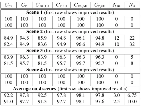
Cm Cr Cm,10 Cr,10 Cm,50 Cr,50 Nm Ns Scene 1(first row shows improved results)
100 100 100 100 100 100 0 0
100 100 100 100 100 100 0 0
Scene 2(first row shows improved results)
84.9 94.8 85.9 94.8 96.1 94.8 12 22
82.4 94.9 83.6 94.9 96.6 94.9 10 32
Scene 3(first row shows improved results)
83.9 96.3 83.9 96.3 96.3 96.3 0 5
81.5 95.7 81.5 95.7 95.7 95.7 0 8
Scene 4(first row shows improved results)
100 100 100 100 100 100 0 0
100 100 100 100 100 100 0 0
Average on 4 scenes(first row shows improved results)
92.2 97.8 92.5 97.8 98.1 97.8 3.0 6.75
91.0 97.7 91.3 97.7 98.1 97.6 2.5 10.0
Table 2: Comparing object-based building detection results in Septemberdata sets with and without the application of the pro-posed improvement. Cm= completeness andCr= correctness (Cm,10,Cr,10andCm,50,Cr,50are for buildings over 10 m
2 and 50 m2
, respectively) are in percentage.Ns= number of split op-erations andNm= number of merge operations.
7. EXPERIMENTAL RESULTS
The experimental results are presented for building detection, change detection and map update separately.
7.1 Building detection results
The performance of the building detection step was evaluated us-ing the object-based completeness and correctness measures, as well as the number of split and merge operations (Awrangjeb and Fraser, 2014a). Split operations are required during evaluation due to under-segmentation errors when two or more buildings are detected as one single building. Conversely, merge operations are required due to over-segmentation errors when a single building is detected as two or more buildings.
Table 2 compares the evaluation results on the September data sets, with and without the application of the proposed improve-ment presented in Section 3.. Table 3 shows the same for the December data sets.
Cm Cr Cm,10 Cr,10 Cm,50 Cr,50 Nm Ns Scene 1(first row shows improved results)
100 86.1 100 86.1 100 86.1 5 3
100 81 100 81 100 81 2 12
Scene 2(first row shows improved results)
92.5 81.7 94.2 81.7 100 81.7 14 60
82.4 60.9 87.5 60.9 100 60.9 0 84
Scene 3(first row shows improved results)
95.2 83.3 95.2 83.3 100 83.3 3 15
100 66.7 100 66.7 100 66.7 0 34
Scene 4(first row shows improved results)
100 100 100 100 100 100 0 0
100 100 100 100 100 100 0 0
Average on 4 scenes(first row shows improved results)
96.9 87.8 97.4 87.8 100 87.8 5.5 19.5
95.6 77.2 96.9 77.2 100 77.2 0.5 32.5
Table 3: Comparing object-based building detection results in Decemberdata sets with and without the application of the pro-posed improvement. Cm= completeness andCr = correctness (Cm,10,Cr,10andCm,50,Cr,50are for buildings over 10 m
2 and 50 m2
, respectively) are in percentage.Ns= number of split op-erations andNm= number of merge operations.
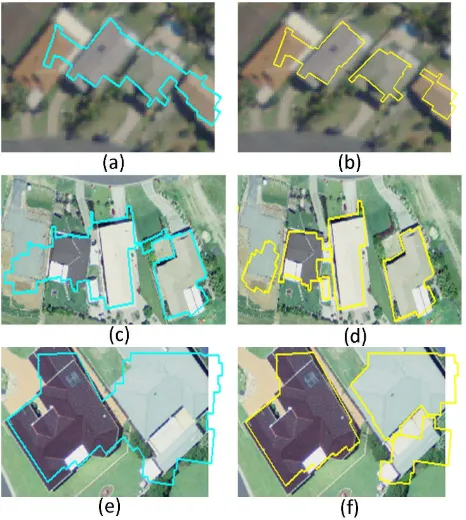
Figure 5: Building detection examples: with (left) and without (right) the improvement in Section 3. Row 1 from Scene 2 and Rows 2 & 3 from Scene 3.
the December data sets where connected building parts were sep-arated (see the example in Fig. 5f, originally together in the ref-erence data set).
Comparing the results from September and December, high com-pleteness values were observed in December due to higher point density, which allowed detection of some small buildings in both Scenes 2 & 3. However, high point density also allowed some detection of trees, which reduced the correctness. This might also be the case because the vegetation became denser during the Spring (Sep-Dec). The number of split operations was lower in September than in December, because low point density data kept the segmented planes from neighbouring buildings further away
Reference Change det. Comm. error Scenes N DP N D NP DP N D NP DP
1 18 1 27 1 1 1 9 1 1 0
2 6 0 18 2 97 66 12 2 97 66
3 3 1 8 0 15 1 5 0 15 0
4 1 0 1 0 0 0 0 0 0 0
Table 4: Change detection results withremoval of commission errors>9 m2 in area. N = new buildings, D = demolished buildings, NP = new building parts and DP = demolished building parts.
Reference Change det. Comm. error Scenes N DP N D NP DP N D NP DP
1 18 1 20 1 1 1 2 1 1 0
2 6 0 10 0 27 11 4 0 27 11
3 3 1 6 0 13 1 3 0 13 0
4 1 0 1 0 0 0 0 0 0 0
Table 5: Change detection results withremoval of commission errors>25 m2
in area. N = new buildings, D = demolished buildings, NP = new building parts and DP = demolished building parts.
Figure 6: Building change detection in Scene 2: larger than (a) 9 m2and (b) 25 m2(small regions removed).
Figure 7: Building change detection in Scene 3: larger than (a) 9 m2and (b) 25 m2(small regions removed).
from each other.
7.2 Change detection results
Tables 4 and 5 show the change detection results for the test scenes. Although, there were no omission errors (missing new and/or demolished buildings and/or building parts), there were a significant number of commission errors (false identification of new and/or demolished buildings and/or building parts), mainly propagated from the building detection step, especially in Scenes 2 & 3.
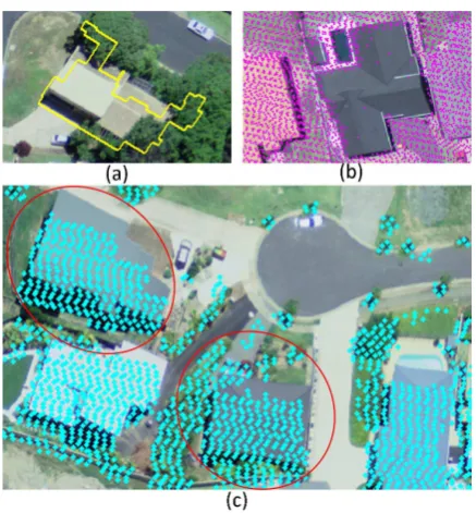
Figure 8: Some difficulties in building detection: (a) extended over the occluding tree, (b) missing building due to absence of point cloud data and (c) registration error between orthoimage and point cloud data in Scene 2.
found to be extended over neighbouring trees (see Fig. 8a) and some trees were detected as separate buildings. There was one false demolished building due to the absence of data in the input point cloud (see Fig. 8b). Also, there were many false demol-ished build parts. This exclusively happened in Scene 2, as shown in Fig. 6a, and was due to registration error between the existing building map, which was manually created from the supplied or-thophoto, and the automatically detected building footprints from the LIDAR point cloud. An example of this registration error is shown within the red circles in Fig. 8c. The registration error also led to some false detection of extended buildings, as shown within orange circles in the magnified version of Fig. 4. However, in the other three scenes the number of false demolished building parts was low because the registration error was negligible. For example, Fig. 7 shows the change detection result for Scene 3.
Scenes D A S M NB EB NM
Table 6: Estimation of manual interactions to generate map using automatically extracted buildings. D = number of deletions for removing false buildings (trees), A = number of additions for in-clusion of missing true buildings, S = number of split operations, M = number of merge operations, NB = number of detected build-ings being edited to be acceptable, EB = number of editions per edited building and NM = number of mouse clicks per edition.
7.3 Map from automatic buildings vs point density
The simple GUI was mainly used for user interaction to quickly accept or reject the suggested changes. Fig. 9a shows the updated
Scenes Cm Cr Ql Ao Ac RM SE
Table 7: Pixel-basedevaluation results forSeptemberdata set for the generated map from the automatically extracted buildings. Cm= completeness,Cr = correctness,Ql= quality,Ao = area omission error andAc= area commission error are in percentage. RM SE= root mean square error in metre.
Scenes Cm Cr Ql Ao Ac RM SE
Table 8: Pixel-basedevaluation results forDecemberdata set for the generated map from the automatically extracted buildings. Cm= completeness,Cr = correctness,Ql= quality,Ao = area omission error andAc= area commission error are in percentage. RM SE= root mean square error in metre.
map for Scene 1.
In the case where a building map is not available for an area, the GUI can also be used to generate a map from the automatically extracted building footprints for that area. Thus, for all eight data sets (4 scenes, each from two dates) new building maps were gen-erated from their extracted footprints via the GUI, with minimum user interaction. False buildings were simply deleted and missing buildings were added. There were also merge and split operations to handle over- and under-segmentation cases. As a final step, a number of edits were required for many buildings to make a vi-sually acceptable building map. Figs. 9b-c show an example for Scene 2, December.
Table 6 shows an estimation of the manual works that was ‘min-imally’ required for the eight data sets. It is evident that the De-cember data required more deletions and more split operations than for the September data, as many trees were detected and many neighbouring buildings were merged. Nevertheless, the December data required less additions since many missing build-ings had been automatically detected because of the higher point density. The four December data sets required less editing and less mouse clicks per edit. This indicates, as could be antici-pated, that detected buildings from a higher density point cloud data contain more detailed information and so require less user interaction.
Table 7 and 8 show pixel-based accuracy for the generated maps (with respect to the manually generated reference buildings). Al-though the maps from two dates showed similar average cor-rectness and commission errors, on average the December maps provided higher completeness and quality and lower omission and geometric errors. Again, better performance is evident with higher density point cloud data.
8. CONCLUSION
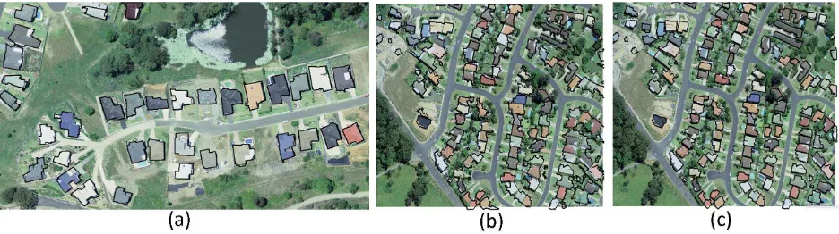
neigh-Figure 9: Map from the extracted buildings: (a) updated map for Scene 1, (b) automatic building detection for Scene 2 in December and (c) map from (b) using the GUI.
bouring buildings in the building mask to avoid any wrong merg-ing of neighbourmerg-ing buildmerg-ings. When compared to the original building detection technique, the improved technique offers not only higher performance in terms of completeness and correct-ness, but also a lower number under-segmentation errors, with a small increase in over-segmentation errors.
An automatic building change detection technique based on con-nected component analysis has also been presented. Buildings which are totally new or demolished are directly added to the change detection output. However, for demolished or extended building parts, a connected component analysis algorithm is ap-plied, and for each connected component its area, width and height are estimated in order to ascertain if it can be considered as a de-molished or extended new building part. Experimental results have shown that the proposed change detection technique pro-vides no omission errors, and thus it can be cheaply exploited for building outline map updating. The resulting high number of commission errors was mainly due to two reasons. Firstly, the building detection technique could not remove all trees and it merged some occluded nearby trees with the detected true build-ings. The high registration error between the exiting map (gener-ated from the orthophotos) also resulted in many false new/demolished building parts. Nonetheless, the commission error does impede the required user interaction, since the user only needs to look at the indicated changes and to accept or reject them. Moreover, this high false change detection of small (new/demolished) build-ing parts is an indication that the proposed detection technique is capable of detecting such real changes in an appropriate data set.
Future research includes reconstruction of building roofs and three dimensional change detection of buildings. While both the point cloud data and high resolution aerial imagery can be used for roof modelling, 3D planes from the point cloud data can be exploited for 3D change detection.
ACKNOWLEDGMENT
Dr. Awrangjeb is the recipient of the Discovery Early Career Researcher Award by the Australian Research Council (project number DE120101778). The Coffs Harbour data set was pro-vided by Land and Property Information of the NSW Government (www.lpi.nsw.gov.au).
REFERENCES
Awrangjeb, M. and Fraser, C. S., 2014a. An automatic and threshold-free performance evaluation system for building ex-traction techniques from airborneLIDARdata. IEEE Journal of Selected Topics in Applied Earth Observations and Remote Sens-ing 7(10), pp. 4184–4198.
Awrangjeb, M. and Fraser, C. S., 2014b. Automatic segmenta-tion of rawLIDARdata for extraction of building roofs. Remote Sensing 6(5), pp. 3716–3751.
Champion, N., Boldo, D., Pierrot-Deseilligny, M. and Stamon, G., 2010. 2d building change detection from high resolution satelliteimagery: A two-step hierarchical method based on 3d in-variant primitives. Pattern Recognition Letters 31(10), pp. 1138– 1147.
Champion, N., Rottensteiner, F., Matikainen, L., Liang, X., Hyyppa, J. and Olsen, B., 2009. A test of automatic building change detection approaches. International Archives of the Pho-togrammetry, Remote Sensing and Spatial Information Sciences XXXVIII(3), pp. 49–54.
Grigillo, D., Fras, M. K. and Petrovic, D., 2011. Automatic ex-traction and building change detection from digital surface model and multispectral orthophoto. Geodetski vestnik 55(1), pp. 28– 45.
Ioannidis, C., Psaltis, C. and Potsiou, C., 2009. Towards a strat-egy for control of suburban informal buildings through automatic change detection. Computers, Environment and Urban Systems 33(1), pp. 64–74.
Matikainen, L., Hyyppa, J., Ahokas, E., Markelin, L. and Kaarti-nen, H., 2010. Automatic detection of buildings and changes in buildings for updating of maps. Remote Sensing 2(5), pp. 1217– 1248.
Murakami, H., Nakagawa, K., Hasegawa, H., Shibata, T. and Iwanami, E., 1999. Change detection of buildings using an air-borne laser scanner. ISPRS Journal of Photogrammetry and Re-mote Sensing 54(2-3), pp. 148–152.
Rottensteiner, F., 2007. Building change detection from digital surface models and multispectral images. International Archives of the Photogrammetry, Remote Sensing and Spatial Information Sciences XXXVI(3/W49B), pp. 145–150.
Vosselman, G., Kessels, P. and Gorte, B., 2005. The utilisation of airborne laser scanning for mapping. International Journal of Applied Earth Observation and Geoinformation 6(3-4), pp. 177– 186.
Zhang, K., Yan, J. and Chen, S. C., 2006. Automatic construction of building footprints from airborne lidar data. IEEE Trans. on Geoscience and Remote Sensing 44(9), pp. 2523–2533.