EXTRACTION OF ICE SHEET LAYERS FROM TWO INTERSECTED RADAR
ECHOGRAMS NEAR NEEM ICE CORE IN GREENLAND
S. Xiong, J.-P. Muller*
Imaging Group, Mullard Space Science Laboratory (MSSL), University College London, Department of Space & Climate Physics, Holmbury St Mary, Surrey, RH5 6NT, UK – [email protected]@ucl.ac.uk
Commission VII/5
KEY WORDS: Cryosphere, Ice sheet layering, Radar echo sounding, Sub-glacial ice flow, NASA IceBridge
ABSTRACT:
Accumulation of snow and ice over time result in ice sheet layers. These can be remotely sensed where there is a contrast in electromagnetic properties, which reflect variations of the ice density, acidity and fabric orientation. Internal ice layers are assumed to be isochronous, deep beneath the ice surface, and parallel to the direction of ice flow. The distribution of internal layers is related to ice sheet dynamics, such as the basal melt rate, basal elevation variation and changes in ice flow mode, which are important parameters to model the ice sheet. Radar echo sounder is an effective instrument used to study the sedimentology of the Earth and planets. Ice Penetrating Radar (IPR) is specific kind of radar echo sounder, which extends studies of ice sheets from surface to subsurface to deep internal ice sheets depending on the frequency utilised. In this study, we examine a study site where folded ice occurs in the internal ice sheet south of the North Greenland Eemian ice drilling (NEEM) station, where two intersected radar echograms acquired by the Multi-channel Coherent Radar Depth Sounder (MCoRDS) employed in the NASA’s Operation IceBridge (OIB) mission imaged this folded ice. We propose a slice processing flow based on a Radon Transform to trace and extract these two sets of curved ice sheet layers, which can then be viewed in 3-D, demonstrating the 3-D structure of the ice folds.
1. INTRODUCTION
Ice sheet layers are principally caused by the accumulation and melting) of snow and ice year by year (Vieli, Siegert, and Payne 2004). The ice sheet layers occur where there is a contrast in electromagnetic properties, and reflect variations of ice density, acidity and fabric orientation from the upper to the lower part of the ice sheets (Fujita et al. 1999). The isochronous and continuous ice layering is very important to understand how the ice sheets respond to past climate change and to forecast its response to future climate change (Vieli, Siegert, and Payne 2004; Morse et al. 1999). On the other hand, the echo-free zone (EFZ) and layer disturbances in the ice sheets are also heated discussed to reflect sub-glacial ice flow at various scales (Drews et al. 2009). Thus, both of the continuity and disturbances of ice sheet layers are indications of ice sheet dynamics, which are very important input parameters to ice sheet modelling and geologic research.
Ice core drilling and ice penetrating radar (IPR) are two methods to acquire information on internal ice sheet layers. Although many geophysical and geochemical parameters can be measured by drilling ice core, it costs a large amount of money, time and field work and only point data can be acquired. IPRs are more efficient though of lower range resolution compared to ice core data. IPRs have been applied to the field of the ice sheet research for more than four decades, and it has wide applications into measurements of surface elevation, ice sheet thickness, snow accumulation rate and bedrock height etc. (Fretwell et al. 2013; Bamber et al. 2013; Gourmelen et al. 2011; Wu et al. 2011; Morse et al. 1999). In order to achieve penetration depths ranging from hundreds to thousands of metres, IPRs are operated at low frequencies ranging from tens to hundreds of Megahertz and employed on the airborne platforms to avoid being affected by the Earth’s ionosphere. The IPRs send radar signals into the ice
*
Corresponding author
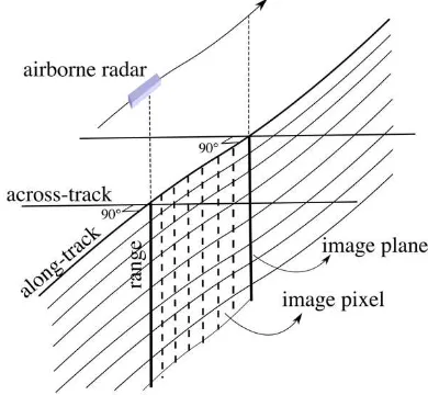
sheet and detect the energy reflected from the ice surface, ice bottom and any englacial targets, generally where there is a contrast in the electromagnetic constitutive properties of the media. Figure 1 shows the imaging geometry of the IPRs.
Figure 1. Imaging geometry of Ice Penetrating Radar (IPR).
ability to show subsurface features interrupting ice sheet layers in three dimensions (along-track, across-track and range direction in Fig. 1). However, few studies have been involved in the reconstruction of vertical structures of the ice sheet layers and horizontal interpolation to restore the terrain of each layer, thus, leading to the reconstruction of 3-D terrain model. In this study, we will attempt to reconstruct the internal ice sheet layers in 3-D, where geometry of subsurface features can be clearly shown. Since tracing and extracting ice sheet layers is the first step to realise the 3-D terrain model, in this paper, we propose an automated detection method for ice sheet layers based on the previous studies. The experiment is carried out with two intersected datasets acquired by the Multi-channel Coherent Radar Depth Sounder (MCoRDS) on board the NASA Operational IceBridge (OIB). In Section 2, the study site and datasets are introduced. In Section 3, we describe the processing methods including the line detection method based on the Radon Transform (RT). Then in Section 4, these are applied to the MCoRDS data and the results are demonstrated. Extraction of ice sheet layers by the method proposed in this paper is concluded in Section 5.
2. STUDY SITES AND DATA
2.1 NEEM Ice Drilling Core
Our study site is located south of the North Greenland Eemian Ice Drilling (NEEM) ice core, where the MCoRDS acquired two intersecting radar echograms, as shown in Fig. 2. The 2 540 m long North Greenland Eemian Ice Drilling (NEEM) ice core was drilled during 2008-2010 through the ice sheet in Northwest Greenland (77.45°N, 51.07°W, surface elevation 2 479 m). The present-day annual snow accumulation at the NEEM site is 0.22 m ice equivalent (Rasmussen et al. 2013). Analysis of several ice- and gas-based records from the NEEM core shows that the lower parts of the core, which contain ice from the Eemian interglacial, have been subject to folding, but no such discontinuities have been identified in the upper 2203.6 m of the core (Dahl-Jensen et al. 2013). The ice layering is disturbed and folded below 2 203.6 m. Below 2 200 m, internal layers become fuzzy and less continuous: undulations and even overturned folds and shearing of basal material are observed. The transition between clear and fuzzy layers often appears at the interface between ice from the glacial and Eemian periods (Dahl-Jensen et al. 2013). The radar images of MCoRDS shows ice folding, which is consistent with ice core results. This demonstrates that radar imaging can now be used to study the folded ice layering.
Figure 2. Study area and the flight track of the IceBridge MCoRDS data used in this study, the elevation data is from
MEaSUREs Greenland Ice Mapping Project (GIMP).
2.2 IceBridge Mission and MCoRDS datasets
The NASA Operation IceBridge is an airborne mission developed to bridge the gap between the Ice, Cloud and Land Elevation Satellite (ICESat), which ceased operation in 2009, and ICESat-2, planned for early 2017. It is the largest airborne survey of the Earth’s polar ice ever flown. It provides the yearly, multi-instrument and 3-D view of Arctic and Antarctic ice sheets, ice shelves and sea ice (Zell 2015). There are several kinds of science instruments installed on IceBridge, including three laser altimeters and five radar instruments. The laser altimeters are mainly used for detecting the surface elevation of ice sheet while the radar sounders are used to view what lies under the ice sheet surface and obtain the elevations of the bedrock.
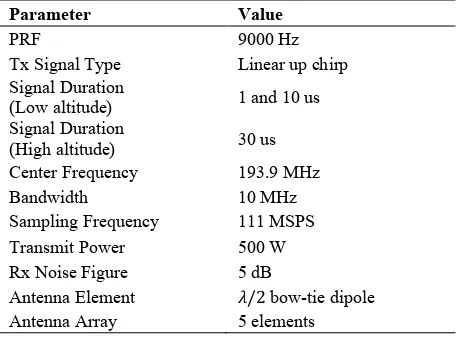
Among the radar sounders employed in OIB, the MCoRDS sensor developed by the Centre for Remote Sensing of Ice Sheets (CReSIS), is a nadir-looking, five channel, monostatic radar system (Shi et al. 2010). It has the lowest frequency, which is supposed to penetrate as deep as several kilometres into the ice sheet in order to reveal the layering of the polar ice sheet. The basic radar parameters of the MCoRDS are shown in Table 1. The IceBridge MCoRDS L1B Geolocated Radar Echo Strength Profiles (IRMCR1B) are radar echograms and they are released in two versions. The first version has temporal coverage from Oct. 16, 2009 to Nov. 06, 2012, and the second from Oct. 12, 2012 to the present. The radar echograms are divided into segments. A segment is a contiguous data set in which the radar settings do not change and each segment is broken into frames, which are generally 50 km long, as shown in Fig. 2.
Table 1. Basic MCoRDS radar parameter (Shi et al. 2010).
Parameter Value
PRF 9000 Hz
Tx Signal Type Linear up chirp Signal Duration
Antenna Element �/2 bow-tie dipole
Antenna Array 5 elements
3. ICE LAYERS DETECTION AND 3D VIEW
3.1 Line Detection and Radon Transform
Tracking continuous isochronal internal layers over the ice sheets for hundreds to thousands of kilometres is difficult due to the occurrence of non-contiguous layers which are related to the local anomaly, such as crevasses and ice folds caused by the internal dynamics of ice sheets. There are many approaches which have been proposed to trace and track internal ice sheet layers from radar echograms. Some of them involve manually digitising layers (Leysinger Vieli, Siegert, and Payne 2004; Morse et al. 1999), but it takes a long time for long profile distance. Interactive semi-automated methods improves the efficiency and insure the accuracy of tracking layers (Macgregor
et al. 2015; Onana et al. 2015; Ferro and Bruzzone 2013). Macgregor et al. (2015) used the phase gradient of radar raw data to detect ice layers, while in many cases, only the radar echograms can be accessed by the public. Ferro and Burzzone (2013) proposed an automatic method to extract layers from SHARAD (Shallow RADar) datasets in the NPLD (North Polar Layer Deposit) of Mars. In this method, filtering was applied to the original dataset before layers extraction in order to improve layer extraction location will be affected. This method also lacks a regularisation step which result in the extracted layer segments not being connected.
The Semi-Automated Multilayer Picking Algorithm (SAMPA) based on the Radon Transform (RT) proposed by Onana et al. in 2015 was applied to extract firn layers detected by the Ku-band radar sounder. The radar echogram is separated into small blocks, assuming that over a short enough distance, a curved layer feature may be approximated with many short line segments, and thus validating the use of the RT (Onana et al. 2015). The theory of a RT is illustrated in Figs. 4 and Fig. 5 which shows an example of RT applied to detect a line in the image. The Radon Transform
�(�, �) of a 2-D image is to sum the pixels � �, � along lines
across the image at different rotation angles .
� �, � = 988 988 � �, � � ����� + ����� − � ���� (1)
where �, � corresponds to a given Cartesian position within the image domain, � ∈ (−∞, ∞) is the distance from the image centre to the line feature, � ∈ [0, �) is the angle between the line feature and the horizontal axis (see Fig. 4 for illustration). The RT is a set of projections along the angular direction, �, of all potential line features from the distance � to the centre of the image. The Cartesian coordinate �, � can be expressed in terms of the local coordinate on the line feature Eq. (2).
� = ����� − � ����
� = ����� + � ���� (2)
Linear features correspond to peaks in the RT domain, thus, straight line segments can be extracted by converting detected peaks in the RT domain back to radar echogram domain. The resultant segmented lines can then be connected and smoothed to form linear features corresponding to ice layers. However, different from the Ku-band radar echogram showing very horizontal firn layers, the radar echogram acquired by MCoRDS shows deeper internal ice sheet layers with larger slope bending, which makes it harder to connect segmented lines converted from detected peaks in the RT domain.
Table 2. File parameter description of IRMCR1B data.
Parameter Description Units
Amplitude Power detected radar echogram data matrix. The first dimension is fasttime and time is the second dimension. Power is relative to the current range line only.
Relative power (log scale)
Fasttime Fast time. Zero time is the time at which the transmit waveform begins to radiate from the
transmit antenna. seconds
Time UTC time of day. This is also known as the slow time dimension. seconds
Elevation WGS-84 geodetic elevation coordinate of the measurement's phase center. Dimension is
time. metres
Surface Estimated two way propagation time to the surface from the collection platform. seconds
Bottom Two way travel time to bottom used during processing. seconds
Latitude WGS-84 geodetic latitude coordinate degrees
Longitude WGS-84 geodetic longitude coordinate degrees
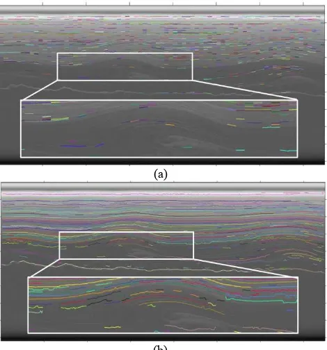
(a)
(b)
Figure 3. Radar echogram along profile (a) AA’ and (b) BB’. Obvious folding structures can be recognised from these
3.2 Ice Layers Extraction and 3D reconstruction
In the SAMPA, the image is divided into blocks and the RT is directly applied to the amplitude of the radar echograms to detect linear features within blocks, and then these segmented linear features can be connected block by block.
Figure 5. An example of RT to detect linear feature.
However, the radar echogram of MCoRDS in this application has a very large gradient in amplitude with those in the upper surface being much stronger than those in the lower pixels. Thus, some peaks are caused by the summation of large value from pixels in the upper rows rather than representing straight lines in the radar echogram at greater depth. For example, this happens when projection carries out along a diagonal line (45° < � < 90°) in the block, as shown in Figs. 5(a) and (b). From Fig. 5(b) we can see that the summations along lines rotated at 45° and 135° are larger than that at 90°, while there is no linear feature along 45° and 135° lines in radar echogram. We tried to adapt this step and applied bilateral filtering (Tomasi and Manduchi 2015), which is an edge remain filtering, adapt histogram equalisation and edge detection before peaks detection in RT domain. This works better than the direct application of RT, but the sensitivity of line detection decreases, thus, causing many gaps of segmented lines and adding difficulties in the following line connection step. Another issue of the SAMPA is that it is suitable for detecting firn layers because of their horizontal orientation, however, when applied to deeper ice sheet layers, such as those in our application, the connection of segments becomes very difficult because connection of segmented lines to form curved layers tends to form horizontal lines, with misconnections as shown in Fig 9(a).
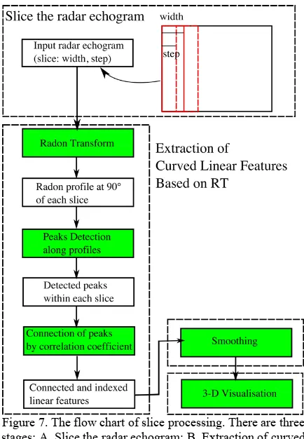
In order to overcome the aforementioned difficulties, we adapt the block processing of the SAMPA into a slice processing method based on the Radon Transform to extract ice sheet layers and apply the calculation of correlation coefficient between peaks within neighbouring slices to connect segmented lines. The proposed slice processing method is illustrated in Fig. 7 and processing steps are described as following.
、 Figure 6. Block processing based on the Radon Transform applied to MCoRDS radar echogram, (a) the original radar echogram; (b) Radon Transform directly applied into original
radar echogram; (c) Bilateral filtering of radar echogram;(d) radar echogram after adaptive histogram equalization; (e) edge detection by the Canny algorithm; (f) Radon Transform of (e),
showing obvious peaks.
Figure 7. The flow chart of slice processing. There are three stages: A. Slice the radar echogram; B. Extraction of curved
linear features based on RT, C. Smoothing and D. 3-D visualisation. (green rectangles indicate the steps, white ones
denote the intermediate results). Figure 4. The illustration of Radon Transform, when the
A. Slice the Radar Echogram. The amplitude of the radar echogram decreases from the surface to the bedrock below, so pixels of the same ice sheet layer have a similar level of amplitude. In order to take advantage of this property and maintain the consistency of layers from the surface to the bottom, we separate the radar echograms into slices along the direction of the flight track rather than into blocks. The width of the sliced image is W pixels. While we detect curved linear features, we move the slice window across the radar echogram along the flight track direction with a step of S pixels. Generally, W can be large, such as 100 pixels in this study, and S should be small enough (S<W), because we are detecting curved lines. The set of W and S is shown in Fig. 7.
B. Extraction of Curved Linear Features Based on RT. Processing at this stage includes applying the Radon Transform, peaks detection along the RT profile, connection of peaks to form linear features. Since the moving step of the slice window is small enough, we can take all the segmented linear features within the slices as horizontal lines. Thus, detection of these horizontal lines can be simplified to detect the peaks along the RT profile at 90°, which is actually the summation of pixel values along horizontal lines, and the location of the peaks along the 90° RT profile corresponds to the y coordinate of the horizontal lines. From the second slice, each peak in this slice is extracted and moved along the previous 90° RT profile. The correlation coefficient is calculated and the maximum of the correlation coefficient indicates a peak in the previous slice to be connected with the current one, as observed in Fig. 8.
Figure 8. The calculation of the correlation coefficient to connect and index peaks, which correspond to the segmented
lines (The black dots on the line are detected peaks).
C. Smoothing of the Extracted Linear Features. After the previous steps, the linear features are extracted and indexed. However, because of the limited sensitivity of peaks detection, there are missing detections of segmented lines in some slices, leading to gaps in the linear features. A smoothing procedure based on the fully automated algorithm developed by (Garcia 2010) is applied to solve this problem. The large gaps between line segments were not filled because this algorithm does not work when filling in gaps for curved parts of lines.
D. 3D visualisation. The y coordinate can be converted to WGS84 elevation using the altitude of the platform, propagation time, and the surface range echo time given in the MCoRDS data file. After conversion of both two radar echograms, they can be
put into a 3-D visualisation to study the vertical structure of the folding ice.
4. RESULTS AND ANALYSIS
Although the SAMPA is not ideal for our application, it was applied on the radar echograms AA’ shown in Fig. 2. In addition, the slice processing method proposed in this paper was applied on the two intersected radar echograms AA’ and BB’ in Fig. 2. In order to demonstrate the effectiveness of the block processing of the SAMPA and slice processing proposed by this paper, we compared the linear features detected by these two methods, which are shown in Fig. 9, from which we can see that the slice processing method (Fig. 9a) can extract curved linear features with a slight merger of layers, while lines detected by block processing are very hard to be connected because the amplitude gradient was not utilised and many gaps appear during line detection by block processing.
(a)
(b)
Figure 9. Comparison between extracted linear features along radar echogram AA’ by (a) block processing and (b) slice processing (block size is 50 × 50 pixels, and slice width is 20
pixels with a step of 6 pixels).
hindered the continuity of line detection by slice processing along this profile.
(a)
(b)
(c)
Figure 10. Results of line detection on the radar echograms: (a) extracted linear features along radar echogram AA’ (slice width of 20 pixels, step of 6 pixels); (b) extracted linear features along radar echogram BB’ (slice width of 20 pixels, step of 6 pixels);
(c) extracted linear features along radar echogram BB’ (slice width of 40 pixels, step of 12 pixels).
The linear features extracted from the two intersected radar echograms are shown in 3-D format, displayed in Fig. 11. From this visualization, we can see that the layers are confirmed between these two profiles. The two intersected radar echograms
imaged the same folded ice in two directions. Along the direction of radar echogram AA’, the ice is folding more intensively than that along the direction of radar echogram BB’. The directions of the folded ice along the two radar echograms are interpreted as arrows in Fig. 11. The dashed arrow line shows the approximate direction after combining the two component directions.
5. CONCLUSIONS AND FUTURE WORK
Detection of ice sheet layers is important to ice sheet studies yet difficult to be achieved with high efficiency and accuracy at the same time. In this paper, we proposed a slice processing method based on a Radon Transform (RT) and applied this to extract and index two sets of intersected ice sheet layers imaged by MCoRDS in Greenland. Compared to previous methods based on block processing, the slice processing flow appears more effective to extract continuous ice sheet layers, especially for deeper ice sheet layers. Visualisation ice sheet layers from intersected radar echograms helps us to study the 3-D structure of the folded ice. The gaps along extracted ice sheet layers indicate the occurrence of anomalies in the ice sheet.
However, the effectiveness of the ice sheet layer detection is qualitatively analysed at this moment, quantitative analyses are needed in the future work. In addition, effective interpolation algorithms for each ice layers and horizontal interpolation of each layer are needed to fill the gaps and smooth the layers, and to combine different profiles to produce a 3D block diagram of the sub-surface. In terms of 3-D structure reconstruction, the connection of the same layers of different flight tracks is needed to be investigated further in the future. Moreover, we plan to look into the co-registration of the surface layer detected by laser altimetry with the surface layer observed in the radar echograms as well as the application of seismic reconstruction techniques to reconstruct subsurface layers.
Figure 11. Linear features extracted from two intersected radar echograms shown in 3-D format.
ACKNOWLEDGEMENTS
We acknowledge support of the CSC and the UCL MAPS Dean prize for the first author. We would also like to thank Anthony Freeman (JPL) for helpful comments.
REFERENCES
Changes in the Weddell Sea Sector of West Antarctica from Radar-Imaged Internal Layering”, Journal of Geophysical Research: Earth Surface, 120(1), pp. 655–670. doi:10.1109/TGRS.2012.2206078.
Dahl-Jensen, D., Albert, M. R., Aldahan, A., Azuma, N., Balslev-Clausen, D., Baumgartner, M., Berggren, A. M., et al., 2013, “Eemian Interglacial Reconstructed from a Greenland Folded Ice Core”, Nature 493 (7433). Macmillan Publishers Limited, 489– 494. doi:10.1038/nature11789.
Ferro, A., and Bruzzone, L., 2013, “Automatic Extraction and Analysis of Ice Layering in Radar Sounder Data”, Geoscience and Remote Sensing, IEEE Transactions on 51 (3), pp. 1622– 1634. doi: 10.1109/TGRS.2012.2206078.
Garcia, D., 2010, “Robust Smoothing of Gridded Data in One and Higher Dimensions with Missing Values”, Computational Statistics & Data Analysis 54 (4), pp. 1167–1178. doi: 10.1109/TGRS.2012.2206078
Karlsson, N. B., Rippin, D. M., Bingham, R. G. and Vaughan, D. G., 2012, “A ‘continuity-Index’ for Assessing Ice-Sheet Dynamics from Radar-Sounded Internal Layers”, Earth and Planetary Science Letters 335-336. Elsevier, pp. 88–94. doi:10.1016/j.epsl.2012.04.034.
Zell, H., 2015, “IceBridge Mission Overview”, https://www.nasa.gov/mission_pages/icebridge/mission/index.ht ml (accessed 06 Apr. 2016)
Leuschen, C., Gogineni, P., Hale, R., Paden, J., Rodriguez, F., Panzer, B., Gomez, D., 2015, “IceBridge MCoRDS L1B Geolocated Radar Echo Strength Profiles, Version 2”, Boulder, Colorado USA: National Snow and Ice Data Center. http://dx.doi.org/10.5067/90S1XZRBAX5N.
Leysinger Vieli, G. J.-M. C., Siegert, M. J and Payne, A. J., 2004, “Reconstructing Ice-Sheet Accumulation Rates at Ridge B, East Antarctica”, Annals of Glaciology 39 (1). International Glaciological Society, pp. 326–30.
Macgregor, J. A., Fahnestock, M. A., Catania, G. A., Paden, J. D., Gogineni, S. P., Young, S. K., Rybarski, S. C., Mabrey, A. N., Wagman, B. W. and Morlighem, M., 2015, “Radiostratigraphy and Age Sturcture of the Greenland Ice Sheet”, Journal of Geophysical Research: Earth Surface 120, pp. 212–41. doi:10.1002/2014JF003215.
Morse, D. L., Waddington, E. D., Marshall, H.-P., Neumann, T. A., Steig, E. J., Dibb, J. E., Winebrenner, D. P. and Arthern, R. J., 1999, “Accumulation Rate Measurements at Taylor Dome, East Antarctica: Techniques and Strategies for Mass Balance Measurements in Polar Environments”, Geografiska Annaler Series A Physical Geography 81 (4), pp. 683–94. doi:10.1111/1468-0459.00106.
Onana, V. D. P., Koenig, L. S., Ruth, J., Studinger, M. and Harbeck, J. P., 2015, “A Semiautomated Multilayer Picking Algorithm for Ice-Sheet Radar Echograms Applied to Ground-Based near-Surface Data”, IEEE Transactions on Geoscience and Remote Sensing 53 (1), pp. 51–69. doi:10.1109/TGRS.2014.2318208.
Rasmussen, S. O., Abbott, P. M., Blunier, T., Bourne, A. J., Brook, E., Buchardt, S. L., Buizert, C., et al., 2013, “A First Chronology for the North Greenland Eemian Ice Drilling (NEEM) Ice Core”, Climate of the Past 9 (6). Copernicus GmbH,
pp. 2713–30. doi:10.5194/cp-9-2713-2013.
Shi, L., Allen, C. T., Ledford, J. R., Rodriguez-Morales, F., Blake, W. A., Panzer, B. G., Prokopiack, S. C., Leuschen, C. J. and Gogineni, S., 2010, “Multichannel Coherent Radar Depth Sounder for NASA Operation Ice Bridge”, In 2010 IEEE International Geoscience and Remote Sensing Symposium, pp. 1729–32. IEEE. doi:10.1109/IGARSS.2010.5649518.