EVALUATION OF FILTERS FOR ENVISAT ASAR SPECKLE SUPPRESSION IN
PASTURE AREA
Xin Wang¹, Linlin Ge¹*, Xiaojing, Li¹²
1.School of Surveying and Spatial Information Systems, 2.School of Civil and Environment Engineering, the University of New South Wales, Sydney, NSW 2052, Australia - [email protected]
Commission VII, WG VII/7
KEY WORDS: ENVISAT ASAR, Speckle noise, filters, ENL, SSI, SMPI
ABSTRACT:
In order to quantify real time pasture biomass from SAR image, regression model between ground measurements of biomass and ENVISAT ASAR backscattering coefficient should be built up. An important prerequisite of valid and accurate regression model is accurate grass backscattering coefficient which, however, cannot be obtained when there is speckle. Speckle noise is the best known problem of SAR images because of the coherent nature of radar illumination imaging system. This study aims to choose better adaptive filter from NEST software to reduce speckle noise in homogeneous pasture area, with little regard to linear feature (e.g. edge between pasture and forest) or point feature (e.g. pond, tree) preservation. This paper presents the speckle suppression result of ENVISAT ASAR VV/VH images in pasture of Western Australia (WA) using four built-in adaptive filters of the NEST software: Frost, Gamma Map, Lee, and Refined Lee filter. Two indices are usually used for evaluation of speckle suppression ability: ENL (Equivalent Number of Looks) and SSI (Speckle Suppression Index). These two, however, are not reliable because sometimes they overestimate mean value. Therefore, apart from ENL and SSI, the authors also used a new index SMPI (Speckle Suppression and Mean Preservation Index). It was found that, Lee filter with window size 7×7 and Frost filter (damping factor = 2) with window size 5×5 gave the best performance for VV and VH polarization, respectively. The filtering, together with radiometric calibration and terrain correction, paves the way to extraction of accurate backscattering coefficient of grass in homogeneous pasture area in WA.
INTRODUCTION
All radar images are inherently corrupted by speckle. The presence of speckle in an image degrades the quality of the image and makes interpretation of features more difficult. Thus, it is often necessary to enhance the image by speckle filtering before data can be used in various applications. More than a dozen of filters have been developed for speckle suppression. All major commercial image processing systems, such as, ER Mapper, PCI EASI/PACE and Erdas/IMAGINE, include a number of image filters for radar speckle comprehensive review of the better-known SAR filters. Sheng and Xia (1996) presented the result of a comprehensive evaluation of filters for radar speckle suppression available in the Erdas/IMAGINE Radar Module. Backscatter signals add to each other coherently and random interference of electromagnetic signals causes the speckle noise to occur in the image (Saevarsson et al., 2004). In fact, speckle is multiplicative noise that alters the real intensity values of features in a scene (Dong et al., 2001). Hence, speckle reduces the potential of SAR images to be utilized as effective data in remote sensing applications such as biomass estimation and interpretation, due to degradation in appearance, quality and the recorded power of returns (Ali et al., 2008; Lee and Pottier, 2009). For this reason, speckle reduction becomes one of the more important tasks in radar remote sensing.
The spatial filters are categorized into two different groups, i.e., non-adaptive and adaptive. Non-adaptive filters take the parameters of the whole image signal into consideration and leave out the local properties of the terrain backscatter or the nature of the sensor. These kinds of filters are not appropriate for non-stationary scene signal. On the other hand, adaptive filters accommodate changes in local properties of the terrain backscatter as well as the nature of the sensor. In these types of filters, the speckle noise is considered as being stationary but the changes in the mean backscatters due to changes in the type of target are taken into consideration. Adaptive filters reduce speckles while preserving the edges (sharp contrast variation). These filters modify the image based on statistics extracted from the local environment of each pixel. Adaptive filter varies the contrast stretch for each pixel depending upon the Digital Number (DN) values in the surrounding moving kernel. Obviously, a filter that adapts the stretch to the region of interest (the area within the moving kernel) would produce a better enhancement. Lee, Gamma Map, and Frost are examples of such filters.
The Lee filter utilizes the statistical distribution of the DN values within the moving kernel to estimate the value of pixel of interest. This filter assumes a Gaussian distribution for the noise in image data. The formula used for the Lee filter is (Lee, 1981):
[ ] [ ]
Where Mean=average of pixels in a moving window
[ ] [ ]
[ ]
The Maximum A Posteriori (MAP) filter is based on a multiplicative noise model with non-stationary mean and variance parameters. The Gamma-Map algorithm assumes a Gamma distribution and its exact formula is the following
The Frost filter replaces the pixel of interest with a weighted sum of the values within the n*n moving kernel. The weighting factors decrease with distance from the pixel of interest. This filter assumes multiplicative noise and stationary noise statistics and follows the following formula:
∑ | |
Like Lee filter, Frost filter is based on the local statistics and the multiplicative model. It differs from the Lee filter in that the scene reflectivity is estimated by convolving the observed image with the impulse response of the SAR system and it averages less in the edge areas to preserve the edge (Sheng and Xia, 1996). Moreover, Frost filter needs to consider the influence of damping factor which determines the amount of exponential damping. Larger damping values preserve edges better but smooth less, and smaller values smooth more. A damping value of 0 results in the same output as a low pass filter.
NEST (Next ESA SAR Toolbox, http://nest.array.ca/web/nest) is a user friendly open source toolbox for SAR image processing from ESA SAR missions including ERS-1 & 2 and ENVISAT. There are four adaptive filters available in NEST: Frost, Gamma Map, Lee, Refined Lee filter. My study aims to extract backscattering coefficient from ENVISAT ASAR APS image in homogeneous pasture area in Western Australia (WA), and a better filter in NEST should be selected to suppress the speckle noise in homogeneous pasture area.
METHODOLOGY
Preparing for extraction of grass backscattering coefficient, this study aims to choose the best filter in NEST software for speckle reduction in homogeneous pasture area, with limited regard to linear feature (e.g. edge between pasture and forest) or point feature (e.g. pond, scattered paddock trees)
preservation. There are two indices usually used for evaluation of speckle suppression ability: ENL (Equivalent Number of Looks) and SSI (Speckle Suppression Index). These two, however, are not reliable when sometimes they overestimate mean value. Therefore, apart from ENL and SSI, we also used a new index SMPI (Speckle Suppression and Mean Preservation Index) to assess the performance of filters. Therefore, ENL, SSI and SMPI were used to assess the smoothing speckle noise over homogeneous areas.
2) Speckle Suppression Index (SSI) This index is based on the equation as follows:
SSI=√
This index tends to be less than 1 if the filter performance is efficient in reducing the speckle noise (Sheng and Xia, 1996). Lower values indicate better performance of speckle filtering.
3) Speckle Suppression and Mean Preservation Index (SMPI)
ENL and SSI are not reliable when the filter overestimates the mean value. We developed an index called Speckle Suppression and Mean Preservation Index (SMPI) (Shamsoddini and Trinder, 2010). The equation of this index is as follow:
pasture area with limited regard to point or linear feature preservation. Therefore, if large area is chosen, classification should be conducted to remove trees, which, however, will
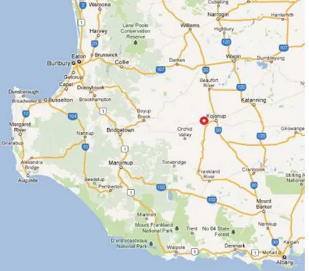
Figure 1, Study area in south west of Western Australia. remove grass under trees and cause discontinuous pasture/grass area, therefore, we cannot choose large area of pasture but a smaller continuous grass area for filter assessment and selection.
RESULTS AND DISCUSSION
ENL, SSI and SMPI were used to assess the performance of filters, and different window sizes were tested: 3*3, 5*5, 7*7 and 9*9. It seems that no filter brings the smallest value of SSI and SMPI and the biggest value of ENL at the same time (Table 1). For example, Frost with 9*9 window and damping factor 3 brings the smallest value for ENL, and GammaMap with 9*9 window gives the smallest SSI. For all filter window sizes (3*3, 5*5, 7*7, 9*9), Lee filter give better performance than GammaMap and Frost filter according to ENL, moreover, the bigger the filter window size, the better the performance. Frost filter with damping factor 1 gives best performance among all three damping factors. Similarly, for all window sizes, Lee gives better performance than Frost according to SSI, and Lee is better than GammaMap for window size 3 and 5, but worse for window size 7 and 9. However, for SMPI, it is more complicated.
ENL and SSI are not reliable when sometimes they overestimate mean value, therefore, SMPI was given the higher priority than ENL and SSI in evaluation of speckle filtering performance. It was found that, for VV polarization, Lee filter with 7×7 window gave the smallest value of SMPI of 2.27, and the third smallest SSI of 0.54 after GammaMap with 9×9 window (0.51) and Lee with 9×9 window (0.52), and Frost filter 7×7 (damping factor=2,1,3) gave the second smallest SMPI: 2.51, 2.72, and 3.23. For VH polarization, Frost filter (damping factor =2) with window size 5×5 gave the smallest value of SMPI 1.25, followed by Frost 5×5 (damping factor=1) (1.53), and Lee filter 5×5 (1.84). It is hard to say which filter is better only from the images filtering effect on ALOS image (L-band) (Shamsoddini et al., 2010), Lee had better performance in reducing filter noise than Frost and Gamma-Map. In addition, Frost filter also performed well in detail preservation, but GammaMap blurs the images. The study of Sheng and Xia (1996) using SIR-C/X-SAR image found that, the filter with better performance in detail preservation and sharpening the edge between meadow and forest is Frost and Lee, it is the same case for the main road, and edge between meadow and arable land, and GammaMap filter blurs the image seriously.
CONCLUSION
Apart from traditional ENL and SSI, a new filter evaluation index SMPI was also used in this study to evaluate the four NEST built-in filters for homogeneous pasture area in Western Australia. It was found that these three indices cannot achieve the best performance simultaneously for different polarization (VV and VH) images of ENVISAT ASAR. According to SMPI as well as ENL and SSI, it was found that Lee filter with window size 7*7 and Frost filter (damping factor = 2) with window size 5*5 gave the best performance in reducing speckle in homogeneous pasture area for VV and VH polarization, respectively. Moreover, according to previous study results, Lee and Frost filter also perform well in detail preservation. The filtering, together with radiometric calibration and terrain correction, paves the way to extraction of accurate backscattering coefficient of grass in homogeneous pasture area in WA.
In this study, only VV and VH polarizations of ENVISAT ASAR images (C-band) were filtered and evaluated, and more polarizations (HH, HV) and wavelengths (e.g. L-band and X-band) can be studied if possible. For researchers in field of forest and agriculture, this new SMPI index can also be studied and compared with traditional SSI and ENL.
ACKNOWLEDGEMENT
Filter
Window
size Polarization Mean
Stand
deviation Covariance SSI SMPI ENL
Noisy image VV 5265.23 5817.54 2.75
VH 1105.31 1181.62 2.56
Lee 3*3 VV 5241.62 2875.32 1.29 0.69 16.86 3.32
VH 1099.07 565.04 1.22 0.69 5.00 3.78
5*5 VV 5270.17 2326.09 0.98 0.60 3.55 5.13
VH 1103.32 437.63 0.97 0.62 1.84 6.36
7*7 VV 5262.05 2021.02 0.81 0.54 2.27 6.78
VH 1103.15 382.95 0.87 0.58 1.84 8.30
9*9 VV 5257.51 1874.25 0.75 0.52 4.55 7.87
VH 1103.89 342.48 0.77 0.55 1.33 10.39
Refined Lee VV 5064.67 2495.93 1.22 0.69 134.25 4.12
VH 1062.74 480.83 1.10 0.68 28.56 4.89
Frost (k=1) 3*3 VV 5244.16 2979.25 1.37 0.71 15.58 3.10
VH 1099.15 586.46 1.30 0.72 5.10 3.51
5*5 VV 5271.27 2513.05 1.12 0.64 4.49 4.40
VH 1104.03 484.56 1.16 0.67 1.53 5.19
7*7 VV 5261.75 2325.67 1.01 0.61 2.72 5.12
VH 1102.57 444.21 1.03 0.64 2.37 6.16
9*9 VV 5258.73 2247.96 0.97 0.59 4.45 5.47
VH 1102.85 426.06 0.97 0.62 2.13 6.70
Frost (k=2) 3*3 VV 5226.07 3685.22 2.08 0.88 34.93 2.01
VH 1094.42 728.29 1.93 0.88 10.32 2.26
5*5 VV 5280.51 3481.79 2.06 0.86 14.09 2.30
VH 1105.71 687.38 2.03 0.89 1.25 2.59
7*7 VV 5263.26 3393.89 1.96 0.84 2.51 2.40
VH 1102.29 677.6 2.02 0.89 3.57 2.65
9*9 VV 5258.34 3383.88 1.93 0.84 6.61 2.41
VH 1102.45 677.12 1.97 0.88 3.39 2.65
Frost (k=3) 3*3 VV 5224.07 4388.58 2.55 0.97 40.60 1.42
VH 1093.26 872.18 2.31 0.96 12.40 1.57
5*5 VV 5282.21 4407.68 2.6 0.97 17.48 1.44
VH 1106.98 879.96 2.47 0.98 2.62 1.58
7*7 VV 5262.88 4423.5 2.55 0.96 3.23 1.42
VH 1102.35 889.04 2.46 0.98 3.88 1.54
9*9 VV 5260.28 4471.1 2.54 0.96 5.72 1.38
VH 1102.47 899.31 2.43 0.98 3.74 1.50
GammaMap 3*3 VV 5127.83 2829.72 1.33 0.71 96.25 3.28
VH 1074.45 562.96 1.38 0.76 23.39 3.64
5*5 VV 5162.84 2266.14 0.98 0.61 61.72 5.19
VH 1074.63 434.59 1.17 0.70 21.42 6.11
7*7 VV 5166.18 1958.77 0.77 0.54 52.94 6.96
VH 1082.38 357.63 0.73 0.55 12.78 9.16
9*9 VV 5132.86 1779.88 0.67 0.51 65.83 8.32
VH 1077.14 317.82 0.65 0.52 14.70 11.49
Table 1, Assessment of speckle suppression ability of Lee, Refined Lee, Frost, and GammaMap filter in homogeneous pasture area. This table shows the statistical characteristics (mean, standard deviation, covariance) and filter evaluation indices (SSI, ENL, SMPI) of images in noisy and filtered images. For Frost filter, different damping factors (k=1, 2, 3) were tried.
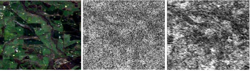
Figure 2, From left to right, from top to bottom: Landsat TM RGB(band3, band2, band1), ENVISAT ASAR VH polarisation: original noisy VH image, VH images filtered by GammaMap, Refined Lee, Frost (damping factor=2), and Lee filter with window size 5*5.
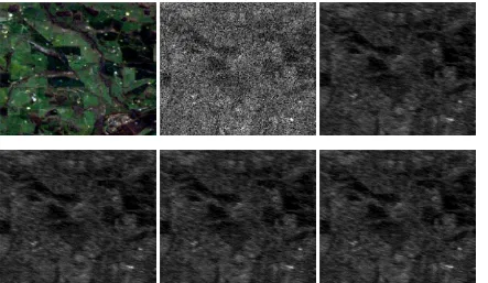
Figure 3, From left to right, from top to bottom: Landsat TM RGB(band3, band2, band1), ENVISAT ASAR VV polarisation original noisy image, VV images filtered by GammaMap, Refined Lee, Frost (damping factor=2), and Lee filter with window size 7*7.
REFERENCES
Durand, J.M., Gimonet, B.J., Perbos, J.R., 1987. SAR data filtering for classification. IEEE Transactions on Geoscience and Remote Sensing, GE-25 (5), pp. 629-637.
Dewaele, P., Wambacq, P., Oosterlinck, A., Marchand, J.I., 1990. Comparison of some speckle reduction techniques for
SAR images. Proceedings of IGARSS’90 Symposium, pp. 2417-2421.
Frost, V. S., Stiles, J. A., Shanmugan, K. S., Holtzman, J. C., 1982. A Model for Radar Images and Its Application to Adaptive Digital Filtering of Multiplicative Noise. Pattern Analysis and Machine Intelligence, IEEE Transactions on, PAMI-4, pp. 157-166.
Gagnon, L., Jouan, A., 1997. Speckle filtering of SAR images: A comparative study between complex-wavelet-based and standard filters. SPIE proceedings, 3169, pp. 80-91.
Kuan, D. T., Sawchuk, A. A., Strand, T. C., Chavel, P., 1985. Adaptive Noise Smoothing Filter for Images with Signal-Dependent Noise. Pattern Analysis and Machine Intelligence, IEEE Transactions on, PAMI-7, pp. 165-177.
Lee, J. S., 1981. Speckle analysis and smoothing of synthetic aperture radar images. Computer Graphics and Image Processing, 17, pp. 24-32.
Lee, J.S., 1983. Digital image smoothing and the sigma filter. Computer Vision, Graphics and Image Processing, 24, pp. 255-269.
Lopes A., Nezry, E., Touzi, R., Laur, H., 1990. Maximum A Posteriori Speckle Filtering and First Order texture Models in SAR Images. International Geoscience and Remote Sensing Symposium (IGARSS).
Qiu, F., Berglund, J., Jensen, J., Thakkar, P., Ren, D., 2004. Speckle Noise Reduction in SAR Imagery Using a Local Adaptive Median Filter. GIScience & Remote Sensing, 41, pp. 244-266.
Rao, P.V.N., Vidyadhar, M.S.R.R., Rao, T.Ch.M., Venkataratnam, L., 1995. An adaptive filter for speckle suppression in synthetic aperture radar images. International Journal of Remote Sensing, 16 (5), pp. 877-889.
Shamsoddini, A., Trinder, J.C., 2010. Image texture preservation in speckle noise suppression. In: Wagner W., Székely, B. (eds.): ISPRS TC VII Symposium – 100 Years ISPRS, Vienna, Austria, July 5–7, 2010, IAPRS, Vol. XXXVIII, Part 7A, pp. 239-244.
Sheng, Y.W., Xia, Z.G., 1996. A comprehensive evaluation of filters for radar speckle suppression. Geoscience and Remote Sensing Symposium, 1996. IGARSS’96. ‘Remote Sensing for a Sustainable Future’, International.
Shi, Z., Fung, K.B., 1994. A comparison of digital speckle filters. Proceedings of IGARSS’94 Symposium, pp. 2129-2133.
Xia, Z.G., Sheng, Y., 1996. Radar speckle: noise or information?