Full Terms & Conditions of access and use can be found at
http://www.tandfonline.com/action/journalInformation?journalCode=ubes20
Download by: [Universitas Maritim Raja Ali Haji] Date: 12 January 2016, At: 17:48
Journal of Business & Economic Statistics
ISSN: 0735-0015 (Print) 1537-2707 (Online) Journal homepage: http://www.tandfonline.com/loi/ubes20
A Simulation-Based Specification Test for Diffusion
Processes
Geetesh Bhardwaj, Valentina Corradi & Norman R Swanson
To cite this article: Geetesh Bhardwaj, Valentina Corradi & Norman R Swanson (2008) A Simulation-Based Specification Test for Diffusion Processes, Journal of Business & Economic Statistics, 26:2, 176-193, DOI: 10.1198/073500107000000412
To link to this article: http://dx.doi.org/10.1198/073500107000000412
Published online: 01 Jan 2012.
Submit your article to this journal
Article views: 76
View related articles
A Simulation-Based Specification Test for
Diffusion Processes
Geetesh BHARDWAJ
Bates and White, San Diego, CA 92130 (geetesh.bhardwaj@gmail.com)
Valentina CORRADI
Department of Economics, University of Warwick, Coventry CV4 7AL, U.K. (v.corradi@warwick.ac.uk)
Norman R. S
WANSONDepartment of Economics, Rutgers University, New Brunswick, NJ 08901 (nswanson@econ.rutgers.edu)
This article makes two contributions. First, we outline a simple simulation-based framework for construct-ing conditional distributions for multifactor and multidimensional diffusion processes, for the case where the functional form of the conditional density is unknown. The distributions can be used, for example, to form predictive confidence intervals for time periodt+τ, given information up to periodt. Second, we use the simulation-based approach to construct a test for the correct specification of a diffusion process. The suggested test is in the spirit of the conditional Kolmogorov test of Andrews. However, in the present context the null conditional distribution is unknown and is replaced by its simulated counterpart. The limiting distribution of the test statistic is not nuisance parameter-free. In light of this, asymptotically valid critical values are obtained via appropriate use of the block bootstrap. The suggested test has power against a larger class of alternatives than tests that are constructed using marginal distributions/densities. The findings of a small Monte Carlo experiment underscore the good finite sample properties of the pro-posed test, and an empirical illustration underscores the ease with which the propro-posed simulation and testing methodology can be applied.
KEY WORDS: Block bootstrap; Finance, continuous time model; Parameter estimation error; Simu-lated GMM; Stochastic volatility.
1. INTRODUCTION
In this article we outline a simple simulation-based frame-work for constructing conditional distributions for multifactor and multidimensional diffusion processes, in the case where the functional form of the conditional density is unknown. The estimated conditional distributions can be used, for example, to form predictive confidence intervals for time period t+τ, given information up to periodt. Further, we use the simulation-based approach to construct tests for the correct specification of a given diffusion model. What distinguishes our approach from that followed by numerous other authors is that we di-rectly evaluate conditional distributions and confidence inter-vals, rather than focusing on marginal and/or joint distributions when constructing our specification test.
Precedents to our article include Corradi and Swanson (CS) (2005a), who constructed various tests, including a Kol-mogorov-type test, based on the comparison of the empirical cumulative distribution function and the cumulative distribu-tion funcdistribu-tion (CDF) implied by the specificadistribu-tion of the drift and the variance functions of a diffusion, and Aït-Sahalia (AS) (1996), who proposed an interesting specification test based on a comparison of the marginal density of the process under the null hypothesis and its kernel counterpart. The AS and CS tests determine whether the drift and variance components of a par-ticular single-factor continuous-time model are correctly speci-fied, although the CS test is based on the comparison of CDFs, whereas Aït-Sahalia’s is based on the comparison of densities, and uses a nonparametric density estimator. The AS test is thus characterized by a nonparametric rate, whereas the CS test has a parametric rate. In the case of multifactor and multidimensional models characterized by stochastic volatility, say, the functional
form of the invariant density of the return(s) is no longer guar-anteed to be given in closed form, upon joint specification of the drift and variance terms, so that the Kolmogorov-type test of CS is no longer applicable. To get around this problem, CS compared the empiricaljointdistribution of historical data with the empiricaljoint distribution of (model) simulated data (see also Corradi and Swanson 2007).
This article is different from that of CS in at least two im-portant ways. First, we provide a correct specification test for a diffusion that is based on the evaluation of an estimate of the
conditionaldistribution, rather than the joint or marginal dis-tribution. This is a relevant departure from CS, because in the literature on the evaluation of continuous-time financial mod-els, the main goal is to construct specification tests based on the transition density associated with a model. In fact, tests based on comparisons of marginal distributions have no power against iid alternatives with the same marginal, for example. Second, we outline an easy-to-implement procedure for con-structing confidence intervals for an asset price for a given pe-riod, sayt+τ. This second feature is important in credit risk management, for example, given that our confidence intervals are predictive intervals whenever the model is estimated using data prior to periodt+1. On the other hand, when models are estimated using all available data, and whent+τ ≤T, then the methods in this article are strictly in-sample, so that our speci-fication test is not ex ante in nature, whereTis the sample size.
© 2008 American Statistical Association Journal of Business & Economic Statistics April 2008, Vol. 26, No. 2 DOI 10.1198/073500107000000412
176
For discussion of theoretical issues that arise when our specifi-cation test is used in ex ante contexts, the reader is referred to Corradi and Swanson (2006a).
If the functional form for the transition density were known, we could test the hypothesis of correct specification of a diffu-sion via the probability integral transform approach of Diebold, Gunther, and Tay (1998), the cross-spectrum approach of Hong (2001), Hong and Li (2005), Hong, Li, and Zhao (2004), and Thompson (2004), the test of Bai (2003) based on the joint use of a Kolmogorov test and a martingalization method, or via the normality transformation approach of Bontemps and Meddahi (2005) and Duan (2003).
Alternative tests to that proposed in this article for the case of unknown transition density functions have recently been sug-gested. For example, Aït-Sahalia, Fan, and Peng (2006) out-lined a test based on the comparison of conditional kernel den-sity estimators and approximations of conditional densities us-ing Hermite polynomials (see also Aït-Sahalia 1999, 2002). In principle, one can also compare conditional kernel density es-timators based on historical and simulated data, along the lines of Altissimo and Mele (2005). One feature of these tests is that they are characterized by nonparametric rates. Our test, on the other hand, is characterized by a parametric rate. This may seem surprising, because it is well known that kernel estimators of conditional distributions converge at nonparametric rates (see, e.g., Fan, Yao, and Tong 1996 and Hall, Wolff, and Yao 1999). Therefore, tests based on the comparison of conditional distrib-utions of simulated and historical data are in general character-ized by nonparametric rates. However, we obtain a parametric rate. This is done by simulatingSpaths of lengthτ,all having as common starting value the observable value at timet,sayXt.
Now, the empirical distribution of the simulated series provides a√T-consistent estimator of the conditional distribution of the null model. We can thus construct a conditional Kolmogorov test, along the lines of Andrews (1997).
Of final note is that the null diffusion model depends on un-known parameters that need to be estimated. Parameters are as-sumed to be estimated via the simulated generalized method of moments (SGMM) approach of Duffie and Singleton (1993), assuming exact identification. This is because√T-consistency does not hold for overidentified (S)GMM estimators of mis-specified models, as shown by Hall and Inoue (2003). Addi-tionally, and as is common with the type of test proposed here, limiting distributions are functionals of zero-mean Gaussian processes with covariance kernels that reflect the contribution of parameter estimation error (PEE). Thus, limiting distribu-tions are not nuisance parameter-free and critical values cannot be tabulated. [Note that in the special case of testing for nor-mality, Bontemps and Meddahi (2005) provided a GMM-type test based on moment conditions that is robust to parameter es-timation error.] In light of this fact, we provide valid asymptotic critical values via an extension of the empirical process version of the block bootstrap which properly captures the contribu-tion of PEE, for the case where parameters are estimated via SGMM. Our bootstrap results stem in part from the fact that when simulation error is negligible (i.e., the simulated sample grows faster than the historical sample), and given exact identi-fication, the results of Gonçalves and White (2004) for QMLE estimators extend to SGMM estimators.
The potential usefulness of our proposed bootstrap-based tests is examined via a series of Monte Carlo experiments using discrete samples of 400 and 800 observations, and based on the use of bootstrap critical values constructed using as few as 100 replications. For the larger sample, rejection rates under the null are quite close to nominal values, and rejection rates under the alternative are generally high. Additionally, an empirical illus-tration is provided which underscores the ease with which one can apply our simulation and testing methodology.
The rest of the article is organized as follows. In Section 2 we outline a setup that is appropriate for discussing our simulation and testing methodology, in the context of one-dimensional dif-fusion processes. In Section 3 we discuss a simple approach to simulation of conditional distributions and confidence intervals. Section 4 outlines our specification test, and Section 5 extends all results to the case of stochastic volatility models. Section 6 contains the results of our small Monte Carlo experiment, and discusses the findings from an empirical illustration based on the Eurodollar deposit rate. Concluding remarks are gathered in Section 7, and all proofs are collected in the Appendix.
2. SETUP
In this section we outline the setup for the case of one-dimensional diffusion processes. All results carry through to the more complicated cases of multidimensional and multifac-tor stochastic volatility models, as outlined in Section 5.
LetX(t),t≥0,be a one-dimensional diffusion process solu-tion to the following stochastic differential equasolu-tion:
dX(t)=μ0(X(t), θ0)dt+σ0(X(t), θ0)dW(t), (1)
whereθ0∈, ⊂ ℜp, andis a compact set. In general,
assume that the model that is specified and estimated is the same as above, but with θ0 replaced by its pseudo true analog,θ†.
Namely, we consider models of the form
dX(t)=μ(X(t), θ†)dt+σ (X(t), θ†)dW(t). (2) Thus, correct specification of the diffusion process corresponds toμ(·,·)=μ0(·,·)andσ (·,·)=σ0(·,·).Note that the drift and
variance terms [μ(·) andσ2(·), respectively] uniquely deter-mine the stationary density, sayf(x, θ†),associated with the in-variant probability measure of the above diffusion process (see, e.g., Karlin and Taylor 1981, p. 241). In particular,
f(x, θ†)= c(θ
†)
σ2(x, θ†)exp
x2μ(v, θ†)
σ2(v, θ†)dv
, (3)
wherec(θ†)is a constant ensuring that the density integrates to 1. However, knowledge of the drift and variance terms does not ensure knowledge of a closed functional form for the transition density.
Now, suppose that we observe a discrete sample (skeleton) of T observations,say (X1,X2, . . . ,XT)′,from the underlying
diffusion. Furthermore, suppose that we use these sample data in conjunction with a simulated “path” to construct an estima-tor ofθ, sayθT,N,h,whereNdenotes the simulation path length
andh is the discretization interval. For the case in which the moment conditions can be written in closed form, and so there is no need of simulations, we have thatθT,N,h=θT. Finally,
note that we use the notation X(t)to denote the continuous-time process, and the notation Xt to denote the skeleton (i.e.,
the discrete sample). In light of this, let Xθt,h denote pathwise simulated data, constructed using someθ∈,and discrete in-tervalh,and sampled at the same frequency of the data.
Assume thatθT,N,h is the simulated generalized method of
moments estimator, which is defined as
θT,N,h=arg min θ∈
1
T T
t=1
g(Xt)− 1 N
N
t=1 g(Xtθ,h)
′ WT
×
1
T T
t=1 g(Xt)−
1
N N
t=1 g(Xtθ,h)
=arg min
θ∈GT,N,h(θ ) ′W
TGT,N,h(θ ), (4)
wheregdenotes a vector ofpmoment conditions,⊂ ℜp(so that we have as many moment conditions as parameters), and
Xtθ,h=Xθ[Kth/N], with N =Kh. Typically the p moment con-ditions are based on the difference between sample moments of historical and simulated data, or between sample moments and model implied moments, whenever the latter are known in closed form. Finally,WT is the inverse of a heteroscedasticity
and autocorrelation (HAC) robust covariance matrix estimator. That is,
WT−1= 1 T
lT
ν=−lT
wν T−lT
t=ν+1+lT
g(Xt)−
1
T T
t=1 g(Xt)
×
g(Xt−ν)−
1
T T
t=1 g(Xt)
′ , (5)
wherewv=1−v/(lT+1).To construct simulated estimators,
we require simulated sample paths. If we use a Milstein scheme (see, e.g., Pardoux and Talay 1985), then
Xθkh−Xθ(k−1)h=b X(θk−1)h, θh+σ X(θk−1)h, θǫkh
−1
2σ X
θ (k−1)h, θ
′
σ Xθ(k−1)h, θh
+1
2σ X
θ (k−1)h, θ
′σ Xθ (k−1)h, θ
ǫkh2, (6)
where(Wkh−W(k−1)h)=ǫkh iid
∼N(0,h),k=1, . . . ,K, Kh= N,andσ (·,·)′is defined later (see Assumption A). Hereafter,
Xkhθ denotes the values of the diffusion at time kh, simulated under θ, and with a discrete interval equal to h, and so is a fine grain analog ofXθt,h. Further, the pseudo true value,θ†, is defined to be
θ†=arg min
θ∈G∞(θ ) ′W
0G∞(θ ),
where G∞(θ )′W0G∞(θ ) =p limN,T→∞,h→0GT,N,h(θ )′WT × GT,N,h(θ ), and whereθ†=θ0,if the model is correctly
spec-ified. Note that the reason why we limit our attention to the ex-actly identified case is that this ensures thatG∞(θ†)=0,even when the model used to simulate the diffusion is misspecified, in the sense of differing from the underlying data generating process (DGP) (see, e.g., Hall and Inoue 2003 for discussion of
the asymptotic behavior of misspecified overidentified GMM estimators). Note also that first-order conditions imply that
∇θG∞(θ†)′W†G∞(θ†)=0.
However, in the case for which the number of parameters and the number of moment conditions is the same,∇θG∞(θ†)′W†
is invertible, and so the first-order conditions also imply that
G∞(θ†)=0.
In the sequel, we shall rely on the following assumption.
Assumption A.
(i) X(t),t∈ ℜ+, is a strictly stationary, geometric ergodic diffusion.
(ii) μ(·, θ†)andσ (·, θ†), as defined in (2), are twice contin-uously differentiable. Also,μ(·,·),μ(·,·)′,σ (·,·),andσ (·,·)′
are Lipschitz, with Lipschitz constant independent ofθ, where
μ(·,·)′ andσ (·,·)′ denote derivatives with respect to the first argument of the function.
(iii) For any fixedhandθ∈,Xkhθ is geometrically ergodic and strictly stationary.
(iv) WT →a.s.W0=−01, where0= ∞
j=−∞E((g(X1)− E(g(X1)))(g(X1+j)−E(g(X1+j)))′).
(v) Hereafter, let∇θXtθ,h be the vector of derivatives with
respect toθ of Xtθ,h.Forθ∈and for allh,g(Xtθ,h)2+δ< C<∞,g(Xθt,h)is Lipschitz, uniformly on, θ→E(g(Xθt,h))
is continuous, andg(Xt),g(Xtθ,h),∇θXθt,hare 2r-dominated (the
last two also on)forr>3/2.
(vi) Unique identifiability:G∞(θ†)′W0G∞(θ†) <G∞(θ )′× W0G∞(θ ),∀θ=θ†.
(vii) θT,N,handθ† are in the interior of,g(Xθt)is twice
continuously differentiable in the interior of , and D† = E(∂g(Xtθ)/∂θ|θ=θ†)exists and is of full rank,p.
Assumption A is rather standard. Assumption A(ii) ensures that under both hypotheses there is a unique solution to the stochastic differential equation in (2). Assumptions A(i) and A(iii)–A(vii) ensure consistency and asymptotic normality of the SGMM estimator.
All results stated in the sequel rely on the following lemma.
Lemma 1. Let Assumption A hold. Assume thatT,N→ ∞.
Then, ifh→0,T/N→0,andh2T→0,then √
T(θT,N,h−θ†) d
→N 0, (D†′W0D†)−1
,
whereW0andD†are defined in Assumptions A(iv) and A(vii).
The above normality result for the SGMM estimator can be ex-tended in a straightforward manner to the case of the EMM es-timator of Gallant and Tauchen (1996) (see also the sequential partial indirect inference approach of Dridi, Guay, and Renault 2006).
3. SIMULATED CONDITIONAL DISTRIBUTIONS
In this section, we outline how to construct in-sampleτ -step-ahead simulated conditional distributions, when the functional form of the conditional distribution is not known in closed form.
Conditional confidence interval construction follows immedi-ately, and is discussed in Section 6. LetSbe the number of sim-ulated paths. Then, fors=1, . . . ,S,t≥1,andk=1, . . . , τ/h,
define
Xsθ,Tt,+Nkh,h −Xsθ,Tt,N,h +(k−1)h
=μ Xsθ,Tt,+N(,hk−1)h,θT,N,h
h+σ Xsθ,Tt+,N,(hk−1)h,θT,N,h
ǫs,t+kh
−1
2σ X
θT,N,h
s,t+(k−1)h,θT,N,h
′σ XθT,N,h
s+(k−1)h,θT,N,h
h
+1
2σ X
θT,N,h
s,t+(k−1)h,θT,N,h ′
σ Xθs,Tt,+N(,hk−1)h,θT,N,h
×ǫs2,t+kh, (7)
whereǫs,t+kh iid
∼N(0,h).That is, we simulateSpaths of length
τ, with τ finite, all having the same starting value, Xt. This
allows for the preservation of the starting value effect on the finite-length simulation paths. It should be stressed, however, that the simulated diffusion is ergodic. Thus, the effect of the starting value approaches zero at an exponential rate, asτ →
∞. Hereafter,XθT,N,h
s,t+khdenotes the value for the diffusion at time t+kh, at simulations,using parametersθT,N,h,a discrete
in-terval equal toh, and using, as a starting value at timet, Xt; Xsθ,Tt,+Nτ,h is defined analogously, by settingkh=τ.
Now, for any given starting value,Xt,the simulated
random-ness is assumed to be independent across simulations, so that
E(ǫs,t+khǫj,t+kh)=0,for alls=j.On the other hand, it is
im-portant to retain the same simulated randomness across differ-ent starting values (i.e., use the same set of random errors for each starting value), so thatE(ǫs,t+khǫs,l+kh)=h,for anyt,l.
Note that the test discussed in the next section requires the construction of multiple paths of length τ, for a number of different starting values, and hence we have attempted to un-derscore the importance of keeping the random errors used in the construction of each set of paths for each starting value the same.
As an estimate for the distribution,at timet+τ,conditional onXt,define
Fτ(u|Xt,θT,N,h)=
1
S S
s=1
1XθT,N,h
s,t+τ ≤u
.
As stated in Proposition 2 below, if the model is correctly specified, then S1Ss=11{Xsθ,Tt,+N,τh ≤u}provides a consistent es-timate of the “true” conditional distribution. A related approach for approximating distribution functions has been suggested by Thompson (2004), in the context of tests for the correct specifi-cation of term structure models. Hereafter, letFτ(u|Xt, θ†)
de-note the conditional distribution ofXtθ+†τ,givenXtθ† =Xt,that
is,Fτ(u|Xt, θ†)=Pr(Xθ
†
t+τ≤u|Xθ
†
t =Xt).
The statement of Proposition 2 requires the following as-sumption.
Assumption B.
(i) Fτ(u|Xt, θ ) is twice continuously differentiable in the
interior of . Also, ∇θFτ(u|Xt, θ ) and ∇θ2Fτ(u|Xt, θ ) are
jointly continuous in the interior of,almost surely, and 2r -dominated on,r>2.
(ii) Xsθ,t+τis continuously differentiable in the interior of,
fors=1, . . . ,S;and∇θXsθ,t+τis 2r-dominated in,uniformly
insforr>2.
Proposition 2. Let Assumptions A and B hold. Assume that
T,N,S→ ∞. Then, if h → 0, T/N → 0, and h2T →0, T2/S→ ∞,the following result holds for anyXt,t≥1,
uni-formly inu:
Fτ(u|Xt,θT,N,h)−Fτ(u|Xt, θ†) pr
→0. (8)
In addition, if the model is correctly specified [i.e., ifμ(·,·)= μ0(·,·)andσ (·,·)=σ0(·,·)]then
Fτ(u|Xt,θT,N,h)−F0,τ(u|Xt, θ0) pr
→0, (9)
whereF0,τ(u|Xt, θ0)=Pr(Xt+τ ≤u|Xt).
In practice, once we have an estimate for theτ-period-ahead conditional distribution, we still do not know whether our esti-mate is based on the correct model. This suggests that one use of the test for correct specification outlined in the next section is to assess the “relevance” of the distribution estimator.
4. SPECIFICATION TESTING
In the first subsection, we outline the test. The second subsec-tion discusses bootstrapping procedures for obtaining asymp-totically valid critical values.
4.1 The Test
The test outlined in this section can be viewed as a simulation-based extension of Andrews (1997) and Corradi and Swanson (2005b, 2006b), which has been adapted to the use of continuous-time models. Of additional note is that in the Andrews and Corradi–Swanson articles, the functional form of conditional distribution under the null hypothesis is assumed to be known, whereas in the current context we replace the con-ditional distribution (or concon-ditional mean) with a simulation-based estimator. Furthermore, in the Andrews article, a condi-tional Kolmogorov test is developed under the assumption of iid data, so that the bootstrap used in that article is not applicable in our context.
Recall that in the previous section we discussed the construc-tion of simulaconstruc-tion paths for a given starting value. To carry out a specification test, however, we now require the construction of a sequence ofT−τ conditional distributions that areτ steps ahead, say. In this way,S paths of lengthτ are thus available for each starting value fromt=1, . . . ,T−τ.
The hypotheses of interest are:
H0:Fτ(u|Xt, θ†)=F0,τ(u|Xt, θ0),for allu,a.s.
HA: Pr(Fτ(u|Xt, θ†)−F0,τ(u|Xt, θ0)=0) >0, for some u∈U,with nonzero Lebesgue measure.
Thus, the null hypothesis coincides with that of correct spec-ification of the conditional distribution,and is implied by the correct specification of the drift and variance terms used in simulating the paths. The alternative is simply the negation of the null. In practice, we observe neither Fτ(u|Xt, θ†) nor F0,τ(u|Xt, θ0).However, we can define the following statistic:
VT= sup
u×v∈U×V|
VT(u,v)|, (10)
where
withUandV compact sets on the real line.
The statistic defined in (10) is a simulation-based version of the conditional Kolmogorov test of Andrews (1997). As stated in Proposition 2, 1SSs=11{XθT,N,h
s,t+τ ≤u}is a consistent
estima-tor of F0,τ(Xt ≤u|Xt, θ0), which is the conditional
distribu-tion implied by the null model. Thus, we compare the joint empirical distribution T−1τTt=−1τ1{Xt+τ ≤ u}1{Xt ≤v} with
its semiempirical/semiparametric analog given by the product of T−1τTt=−1τF0,τ(u|Xt, θ0)1{Xt ≤v}. Intuitively, if the null
model used for simulating the data is correct, then the differ-ence between the two approaches zero, and has a well-defined limiting distribution when properly scaled. The asymptotic be-havior ofVT is described by the following theorem.
Theorem 3. Let Assumptions A and B hold. Assume that
T,N,S→ ∞.Then, ifh→0,T/N→0,T/S→0,T2/S→
where Z(u,v) is a Gaussian process with covariance kernel
K(u,u′,v,v′)given by EXdenotes the expectation under the law governing the sample
andES denotes the expectation under the measure governing
the simulated randomness.
Furthermore, underHA,there exists someε >0 such that
lim
Notice that the limiting distribution is a zero-mean Gaussian process, with a covariance kernel given byK(u,u′,v,v′).The first term is the long-run variance we would have if we knew
F0,τ(u|X1, θ0);the second term captures the contribution of
pa-rameter estimation error; and the third term captures the cor-relation between the first two. As T/S→0, the contribution
of simulation error is asymptotically negligible. The limiting distribution is not nuisance parameter-free and hence critical values cannot be tabulated. In the next section we thus outline a bootstrap procedure for calculating asymptotically valid critical values forVT.
4.2 Bootstrap Critical Values
Given that the limiting distribution of VT is not nuisance
parameter-free, our approach is to construct bootstrap criti-cal values for the test. To show the first-order validity of the bootstrap, we shall obtain the limiting distribution of the boot-strapped statistic and show that it coincides with the limiting distribution of the actual statistic, underH0. Then, a test with
correct asymptotic size and unit asymptotic power can be ob-tained by comparing the value of the original statistic with boot-strapped critical values.
Asymptotically valid bootstrap critical values for the test should be constructed as follows:
Step 1. At each replication, draw b blocks (with replace-ment) of length l, where bl=T. Thus, each block is equal
ries consists ofb blocks that are discrete iid uniform random variables, conditional on the sample. Use these data to construct
θT∗,N,h. ForN/T→ ∞,GMM and simulated GMM are asymp-totically equivalent. Thus, we do not need to resample simu-lated moment conditions. More precisely, define
θT∗,N,h=arg min
Step 2. Using the same set of random errors used in the
con-struction of the actual statistic, constructXθ
∗
T,N,h
s,t+τ,∗,s=1, . . . ,S
andt=1, . . . ,T−τ. Note that we do not resample the simu-lated series (asS/T→ ∞,simulation error is asymptotically negligible). Instead, simply simulate the series using bootstrap estimators and using bootstrapped values as starting values.
Step 3. Construct the following bootstrap statistic, which is the bootstrap counterpart ofVT:
VT∗= sup
−√ 1
Step 4. Repeat Steps 1–3Btimes, and generate the empirical distribution of theBbootstrap statistics.
Note that the first term on the right side of (13) is the boot-strap analog of (11). However, simulation error is asymptoti-cally negligible (asT/S→0),so that there is no need to resam-ple the simulated data. Though, to properly mimic the contribu-tion of parameter estimacontribu-tion error, data are simulated using the bootstrap estimator. Also, we need to use resampled observed values as starting values for the simulated series. The second term on the right side of (13) is the mean of the first, computed under the law governing the bootstrap, and conditional on the sample. It plays the role of a recentering term.
For the iid case when the conditional distribution,F0(yt|Xt),
is known in closed form, Andrews (1997) suggested using a parametric bootstrap procedure [i.e., resample y∗t, say, from
F(u|Xt,θT), keeping the conditioning variates, Xt, fixed]. In
our dynamic context, the conditioning variables cannot be kept constant. One possibility, for the case where τ =1,
would be to draw X∗2 from 1SsS=11{XsθT,N,h(X1)≤u}, sim-this bootstrap procedure may not properly mimic the contribu-tion of parameter estimacontribu-tion error. We leave this issue to future research.
Theorem 4. Let Assumptions A and B hold. Assume that
T,N,S→ ∞.Then, ifh→0,T/N→0,T/S→0,T2/S→
whereP∗ denotes the probability law of the resampled series, conditional on the sample.
The above results suggest proceeding in the following man-ner. For any bootstrap replication, compute the bootstrap statis-tic,VT∗.PerformBbootstrap replications (Blarge) and compute the quantiles of the empirical distribution of theBbootstrap sta-tistics. RejectH0ifVT is greater than the(1−α)th percentile.
Otherwise, do not reject.Now, for all samples except a set with probability measure approaching zero,VThas the same limiting distribution as the corresponding bootstrapped statistic, ensur-ing asymptotic size equal to α.Under the alternative, VT
di-verges to (plus) infinity, whereas the corresponding bootstrap statistic has a well-defined limiting distribution, ensuring unit asymptotic power.
5. STOCHASTIC VOLATILITY MODELS
We now focus our attention on stochastic volatility models. Extension to general multifactor and multidimensional models
follows directly. Consider the following model:
whereW1,t andW2,t are independent standard Brownian
mo-tions, and where μ1(·,·), μ2(·,·),σ11(·,·),σ21(·,·),σ22(·,·),
and θ† are replaced with μ1,0(·,·), μ2,0(·,·), σ11,0(·,·),
σ21,0(·,·), σ22,0(·,·), and θ0, respectively, under correct
spec-ification.
In the one-dimensional case, X(t) can be expressed as a function of the driving Brownian motion, W(t). However, in the multidimensional case, that is X(t)∈Rp, X(t) cannot in general be expressed as a function of the pdriving Brownian motions, but is instead a function of (Wj(t),
t
0Wj(s)dWi(s)), i,j=1, . . . ,p (see, e.g., Pardoux and Talay 1985, p. 30–32). For this reason, simple approximation schemes like the Euler and Milstein schemes, which do not involve approximations of stochastic integrals, may not be adequate. One case in which the Milstein scheme does straightforwardly generalize to the multi-dimensional case is when the diffusion matrix is commutative. Namely, write the diffusion matrix(X)as
(X)=( σ1(X) · · · σP(X) ) ,
then(X)is commutative.
However, almost all frequently used stochastic volatility (SV) models violate the commutativity property (see, e.g., the GARCH diffusion model of Nelson 1990; Heston 1993; and the general eigenfunction stochastic volatility models of Meddahi 2001). A simple way of imposing commutativity is to assume no leverage. Now, the nonleverage assumption is suitable for exchange rates, but not for stock returns. In this situation, more “sophisticated” approximation schemes are necessary.
It is immediate to see that the diffusion in (14) violates the commutativity property. Now, let
and define the following generalized Milstein scheme [see, Kloeden and Platen 1999, p. 346, eq. (3.3)]:
X(θk+1)h=Xkhθ +μ1(Xkhθ , θ )h+σ11(Vkhθ , θ )ǫ1,(k+1)h
V(θk+1)h=Vkhθ +μ2(Vkhθ , θ )h+σ22(Vkhθ , θ )ǫ2,(k+1)h
The last terms on the right side of (16) involve stochastic integrals and cannot be explicitly computed. However, they can be approximated, up to an error of ordero(h), by [see, Kloeden and Platen 1999, p. 347, eq. (3.7)]
(k+1)h
To construct conditional distributions, given the observable state variables, we need to perform the following steps.
Step 1. Simulate a path of length N using the schemes in (16), (17) and estimate θ by SGMM, as in (4). Also, retrieve
VkhθT,N,h,fork=1/h, . . . ,K/h,withKh=N,and hence obtain
Vjθ,Th,N,h,j=1, . . . ,N(i.e., sample the simulated volatility at the same frequency as the data).
Step 2. Using the schemes in (16), (17), simulateS×Npaths of length τ, setting the initial value for the observable state variable to beXt.As we do not observe data on volatility, use
the values simulated in the previous step as the initial value for the volatility process (i.e., as initial values for the unobservable state variable, useVjθ,Th,N,h,j=1, . . . ,N). Also, keep the
sim-constant acrossjandt(i.e., constant across the different start-ing values for the unobservable and observable state variables). DefineXθT,N,h
j,s,t+τ to be the simulated τ-step-ahead value for the
return series at replications,using initial valuesXtandV
initial value of the volatility process, we have integrated out its effect. In other words, 1SSs=11{X
Step 4. Construct the statistic of interest:
SVT= sup
Assumption A′. This assumption is the same as Assump-tion A, except that AssumpAssump-tion A(ii) is replaced by (ii′):μ(·,·)
andσ (·,·)[as defined in (14) and (15)], andσlj(V, θ )∂σkι∂(VV,θ )
are twice continuously differentiable, Lipschitz, with Lipschitz constant independent ofθ,and grow at most at a linear rate, uniformly in, forl,j,k, ι=1,2.
All of the results outlined in Sections 3 and 4 generalize to the current setting. In particular, the following results hold.
Proposition 5. Let Assumptions A′and B hold. Assume that
T,N,S→ ∞. Then, if h→0, T/N→0, T2/S→ ∞, and
In addition, if the model is correctly specified, that is, if
μ(·,·)=μ0(·,·)andσ (·,·)=σ0(·,·),then
In the sequel, consider testing the hypotheses given in Sec-tion 4.1. However, in the present context correct specificaSec-tion of the conditional distribution ofXt+τ|Xtno longer implies correct
specification of the underlying diffusion process. Indeed, cor-rect specification of the stochastic volatility process is equiva-lent to correct specification ofXt+τ,Vt+τ|Xt,Vt.Also, although XtandVtare jointly Markovian,Xtis no longer Markov.
There-fore, by using onlyXt as a conditioning variable, we
implic-itly allow for dynamic misspecification under the null. Further-more, it thus follows that the test has no power against diffusion processes having the same transition density asXt+τ|Xt.
Theorem 6. Let Assumptions A′ and B hold. Assume that
T,N,S→ ∞.Then, ifh→0,T/N→0,T/S→0,T2/S→
where SZ(v) is a Gaussian process with covariance kernel
SK(v,v′)given by
+μSVf0,τ(u,v)′(D0′W0D0)−1μSVf0,τ(u,v)
andEj,sdenotes the expectation with respect to the joint
prob-ability measure governing the simulated randomness and the volatility process,Vθ0
h,j, conditional on the sample.
Furthermore, underHA,there exists someε >0 such that
lim
Note that in a Bayesian context, Chib, Kim, and Shephard (1998) and Elerian, Chib, and Shephard (2002) suggested like-lihood ratio tests for the comparison of a stochastic volatility model against a specific alternative model, for the discrete and continuous cases, respectively. In their tests, the likelihood is constructed via the joint use of probability integral transform and particle filtering (see also Pitt and Shephard 1999; Pitt 2005). These tests differ from ours, as we are interested in as-sessing whether the conditional density ofXt+τ|Xt implied by
the null model is correct.
To obtain asymptotically valid critical values, resample as discussed above for the one-factor model, and note that there is no need to resampleVhθ,j.In particular, form bootstrap statis-tics as follows:
values.This allows us to state the following theorem.
Theorem 7. Let Assumptions A′ and B hold. Assume that
T,N,S→ ∞.Then, ifh→0,T/N→0,T/S→0,T2/S→
∞,Nh→0,h2T→0,l→ ∞,andl2/T→0,the following result holds underH0:
P
As in the single-factor case, the above results suggest pro-ceeding in the following manner. For any bootstrap replication, compute the bootstrap statistic,SV∗T.PerformBbootstrap repli-cations (B large) and compute the quantiles of the empirical distribution of theB bootstrap statistics. RejectH0, ifSVT is
greater than the(1−α)th percentile. Otherwise, do not reject.
Now, under the null, for all samples except a set with probabil-ity measure approaching zero,SVTandSV∗Thave the same
lim-iting distribution, ensuring asymptotic size equal toα.Under the alternative,SVT diverges to (plus) infinity, whereas the
cor-responding bootstrap statistic has a well-defined limiting distri-bution, ensuring unit asymptotic power.
6. EXPERIMENTAL AND EMPIRICAL RESULTS
In this section, we briefly illustrate the above testing method-ology for the case in which we are interested in specification testing from the perspective of conditional confidence intervals. In particular, considerVT=supv∈V|VT(v)|, where
Additionally, define the following bootstrap statistic: VT∗ =
supv∈V|VT∗(v)|,where
It is immediate to see that the above statistic is a version of the distributional test discussed above, so that all of the theo-retical results outlined in Sections 4 and 5 hold. For the case of stochastic volatility models, consider the statistic SVT =
supv∈V|SVp(v)|,where
and its bootstrap analogSV∗T=supv∈V|SV∗T(v)|,where
SV∗T(v)=√ 1 T−τ
T−τ
t=1
1
NS N
j=1 S
s=1
1u≤Xθ
∗
i,T,N,h
j,s,t+τ,∗≤u
−1{u≤X∗t+τ≤u}
1{X∗t ≤v}
−√ 1
T−τ T−τ
t=1
1
NS N
j=1 S
s=1
1u≤Xjθ,is,T,t,+N,τh≤u
−1{u≤Xt+τ≤u}
1{Xt≤v}.
In the sequel we shall study a common version of the square root process discussed in Cox, Ingersoll, and Ross (CIR) (1985), the square root stochastic volatility model of Heston (1993), called SV, and a stochastic volatility model with jumps, called SVJ. The specifications of these models are as follows:
CIR: dr(t)=kr(r−r(t))dt+σr√r(t)dWr(t), wherekr>0, σr>0, and 2krr≥σr2,
SV: dr(t)=kr(r−r(t))dt+√V(t)dWr(t), and dV(t)= kv(v−V(t))dt+σv√V(t)dWv(t),whereWr(t)andWv(t)are
independent Brownian motions, and where kr >0, σr >0, kv>0, σv>0, and 2kvv> σv2.
SVJ: dr(t) = kr(r − r(t))dt +√V(t)dWr(t) + Judqu − Jddqd, anddV(t)=kv(v−V(t))dt+σv√V(t)dWv(t),where Wr(t)andWv(t)are independent Brownian motions, and where
kr>0, σr>0,kv>0, σv>0, and 2kvv> σv2.Further,quand qdare Poisson processes with jump intensityλuandλd,and are
independent of the Brownian motionsWr(t)andWv(t).Jump sizes are iid and are controlled by jump magnitudesζu, ζd>0,
which are drawn from exponential distributions, with densities
f(Ju)=ζ1
uexp(−
Ju
ζu)andf(Jd)=
1 ζdexp(−
Jd
ζd).Here,λuis the
probability of a jump up, Pr(dqu(t)=1)=λu, and jump-up
size is controlled byJu, whereasλdandJdcontrol-jump down
intensity and size. Note that the case of Poisson jumps with constant intensity and jump size with exponential density is covered by the assumptions stated in the previous sections.
6.1 Monte Carlo Experiment
In this subsection, parameterizations for the above models were selected via examination of models estimated using the interest rate data discussed in the next subsection, and include: CIR—(kr,r, σr) = {(.15, .05, .10), (.30, .05, .10), (.50, .05, .10)}; SV—(kr,r,kv,v, σv) = (.30, .05,5.00, .0005, .01);
SVJ—(kr,r,kv,v, σv, λu, ζu, λd, ζd) = (.30, .05,2.5, .0005, .01,8.00, .001,1.50, .001). Note that kr in the data was
es-timated to be approximately .30, and our DGPs set kr = .15, .30, .5. Thus, we include a case where there is substan-tially less mean reversion than that observed in the data. For a discussion of the crucial issue of persistence and its effect on tests related to that discussed in this paper, the reader is re-ferred to Pritsker (1998). Note that the parameters estimated for the three models, ordered as CIR, SV, and SVJ, are kr= .31, .24, .50; r=.068, .059, .068; σr=.11; kv=5.12,1.56; v=.0003, .0009; σv =.014, .029; λu =7.86; ζu =.0004;
λd=2.08;andζd=.0008. Data were generated using the
Mil-stein scheme discussed earlier withh=1/T, forT= {400,800}. The jump component can be simulated without any error, be-cause of the constancy of the intensity parameter.
The three models we study (i.e., the CIR, SV, and SVJ mod-els) fall in the class of affine diffusions. Therefore, it is pos-sible to compute in closed form the conditional characteristic function; for the CIR model we follow Singleton (2001), for the SV model Jiang and Knight (2002), and for the SVJ model Chacko and Viceira (2003). Given the conditional characteris-tic function, we compute as many conditional moments as the number of parameters to be estimated and thus we implement exactly identified GMM. (Note that the criticism of Andersen and Sorensen 1996 about the use of exact GMM does not nec-essarily apply to the case of conditional moments obtained via the conditional characteristic function.)
In our experiment, all empirical bootstrap distributions were constructed using 100 bootstrap replications, and critical val-ues were set equal to the 90th percentile of the bootstrap dis-tributions. For the bootstrap, block lengths of 5, 10, 20, and 50 were tried. Additionally, we setS= {10T,20T},and for mod-els SV and SVJ we setN=S.Tests were carried out usingτ -step-ahead confidence intervals, forτ = {1,2,4,12}, and we set
(u,u);X±.5σX, andX±σX, whereXandσXare the mean and
variance of an initial sample of data. Finally,[v,v]was set equal to[Xmin,Xmax], and a grid of 100 equally spaced values for v
across this range was used, whereXminandXmaxare again fixed
using the initial sample. All results are based on 500 Monte Carlo iterations.
Results are gathered in Tables 1–3. Tables 1 and 2 report re-sults for the size of the test and Table 3 reports rere-sults based on power experiments. In the size experiments, estimated models are the same as the models used for data generation, whereas in the power experiments, we estimate the CIR model when data are generated according to either the SV or SVJ model [Bhardwaj, Corradi, and Swanson 2005 also consider Ornstein– Uhlenbeck (OU) models]; and we estimate an OU model when data are generated according to a CIR model. Finally, for the power experiment where data are generated according to a CIR model, we report results for the parameterization where(kr,r, σr)=(.30, .05, .10) (additional results are available upon
re-quest).
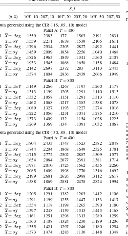
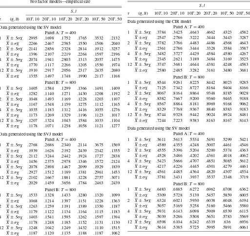
Each of the panels in the tables contains results forT=400 andT=800. Table 1 reports the empirical size for the three CIR parameterizations,whereas Table 2 reports the empirical size for the SV and SVJ models. Turning first to Tables 1 and 2, note that for T =400,empirical size ranges from 13% to 30% (the nominal size is 10%).Additionally, the test seems to perform slightly worse for the SVJ model, whereas there are no relevant differences across the three CIR parameterizations and the SV model. When the sample is increased toT=800 observations, empirical size is rather closed to nominal size, ranging from 10% to 15% (again, there are no obvious differ-ences across different models and parameterizations). Turning now to Table 3, note that rejection rates are rather similar for both cases where data are generated using the SV and the SVJ models. Namely, forT=400 rejection rates range from 35% to 60%,whereas forT =800 rejection rates range from 55% to 75%.Interestingly, these findings seem to be quite robust to the choice of bootstrap block length, as well as to the choice ofS
andτ.
Table 1. Specification test rejection frequencies for the one-factor model—empirical size
S,l
τ (u,u) 10T,10 20T,10 10T,20 20T,20 10T,50 20T,50
Data generated using the CIR(.15, .05, .10)model Panel A:T=400
1 X±.5σX .1559 .2383 .177 .1503 .2191 .2831 X±σX .1559 .2211 .1638 .1539 .2105 .1611
2 X±.5σX .1796 .2534 .2303 .2827 .1492 .1441 X±σX .1459 .2009 .1854 .2256 .1040 .1468
4 X±.5σX .1826 .1963 .1849 .1341 .1560 .2107 X±σX .1933 .1545 .1868 .1658 .1158 .1484
12 X±.5σX .2142 .2697 .2372 .283 .3113 .2443 X±σX .1374 .1804 .2836 .2439 .2666 .1949
Panel B:T=800
1 X±.5σX .1149 .1266 .1267 .1197 .1260 .1177 X±σX .1313 .1199 .1203 .1291 .1110 .1513
2 X±.5σX .1332 .1058 .1151 .1291 .1313 .1110 X±σX .1462 .1068 .1217 .1383 .1388 .1078
4 X±.5σX .1089 .1327 .1193 .1227 .1274 .1016 X±σX .1222 .1056 .1231 .1071 .1275 .1210
12 X±.5σX .1373 .1409 .132 .1154 .1028 .1225 X±σX .1269 .1369 .134 .1091 .1032 .1067
Data generated using the CIR(.30, .05, .10)model Panel A:T=400
1 X±.5σX .1804 .2433 .1747 .1523 .2382 .2848 X±σX .1744 .2204 .1868 .1649 .2325 .1781
2 X±.5σX .1715 .2772 .2502 .2887 .1509 .1577 X±σX .1654 .2084 .2077 .2391 .1381 .1714
4 X±.5σX .1971 .2010 .1725 .1562 .1455 .2260 X±σX .2085 .1609 .1998 .1770 .1316 .1692
12 X±.5σX .2199 .2681 .2626 .2988 .3112 .2617 X±σX .1588 .1869 .2881 .2478 .2824 .1994
Panel B:T=800
1 X±.5σX .1205 .1291 .1382 .1203 .1412 .1106 X±σX .1291 .1199 .1253 .1447 .1133 .1417
2 X±.5σX .1354 .1118 .1198 .1265 .1390 .1180 X±σX .1397 .1248 .1139 .1313 .1443 .1168
4 X±.5σX .1161 .1251 .1298 .1313 .1289 .1259 X±σX .1363 .1108 .1324 .1230 .1189 .1206
12 X±.5σX .1355 .1421 .1297 .1246 .1180 .1254 X±σX .1373 .1474 .1283 .1130 .1148 .1348
6.2 Empirical Illustration
In this subsection, the CIR, SV, and SVJ models discussed above were fit to the 1-month Eurodollar deposit rate for the period January 6, 1971–September 30, 2005 (1,813 weekly ob-servations). Other interest rate datasets examined in the litera-ture include the monthly federal funds rate (Aït-Sahalia 1999), the weekly 3-month T-bill rate (Andersen, Benzoni, and Lund 2004), and the weekly U.S. Dollar swap rate (Dai and Singleton 2000), to name but a few.
We use the specification tests outlined in Section 6.1. In-tervals examined, block lengths considered, simulation sample sizes used, bootstrap replications, and values ofτ considered are the same as discussed in the previous subsection. For exam-ple, we again considerτ= {1,2,4,12}, corresponding to one-week, two-one-week, one-month, and one-quarter-ahead intervals.
Table 1. (Continued)
S,l
τ (u,u) 10T,10 20T,10 10T,20 20T,20 10T,50 20T,50
Data generated using the CIR(.50, .05, .10)model Panel A:T=400
1 X±.5σX .2011 .247 .1886 .1633 .244 .2842 X±σX .1908 .2383 .1944 .1814 .2403 .1756
2 X±.5σX .1904 .2783 .2492 .2978 .1452 .1666 X±σX .1781 .219 .2175 .261 .1547 .181
4 X±.5σX .2141 .2109 .1868 .1783 .1563 .2221 X±σX .2204 .1593 .2075 .2005 .1523 .1977
12 X±.5σX .2257 .2766 .2767 .3171 .3345 .2653 X±σX .162 .1917 .3012 .2662 .2962 .2035
Panel B:T=800
1 X±.5σX .1261 .1368 .1615 .1324 .1568 .1215 X±σX .118 .1248 .1381 .1469 .1225 .1682
2 X±.5σX .1437 .1378 .1231 .1483 .1608 .1209 X±σX .1625 .1429 .1124 .1553 .1585 .1202
4 X±.5σX .1319 .1248 .1451 .1525 .1388 .1541 X±σX .1428 .1263 .1517 .1317 .1364 .1167
12 X±.5σX .1406 .1432 .128 .1202 .145 .1293 X±σX .1399 .1688 .1409 .1216 .1305 .1294
NOTE: Entries in the table are empirical rejection frequencies for tests constructed using intervals given in the second column of the table, and forτ=1,2,4,12. (S,l) combinations used in test construction are given in the second row of the table, so that simulation periods considered areS=(10T,20T)and block lengths considered arel=(10,20,50), where
Tis the sample size, andT=400,800. Empirical bootstrap distributions are constructed using 100 bootstrap replications, and critical values are set equal to the 90th percentile of the bootstrap distribution. Finally,XandσXare the mean and variance of an initial sample
of data. All results are based on 500 Monte Carlo simulations. See Section 6.1 for further details.
The exception is that the interval endpoints are chosen using actual interest rate data (i.e.,X, σX,Xmin,andXmax are
con-structed using the historical data). Note, for example, that using this approach, X±.5σX and X±σX correspond to intervals
with 46.3% and 72.4% coverage, respectively. In the tables, test statistic values (denoted by VT for CIR and SVT for SV and
SVJ) and 5%, 10%, and 20% nominal size bootstrap critical values are given. Single, double, and triple starred entries de-note rejection using 20%,10%,and 5% size tests, respectively. Not surprisingly, the CIR model is rejected using 5% size tests in almost all cases. The same finding has been found, for ex-ample, by Aït-Sahalia (1996) and Bandi (2002). On the other hand, for the SV and SVJ models the results are more mixed. Rejections tend to occur only for the smaller confidence inter-val. Additionally, the SVJ model appears to be rejected slightly more frequently.
7. CONCLUDING REMARKS
In this article we outline a simple simulation-based frame-work for constructing conditional distributions for multifactor and multidimensional diffusion processes, for the case where the functional form of the conditional density is unknown. In a Monte Carlo experiment and an empirical illustration, we show how the estimated distributions can be used, for example, to form conditional confidence intervals for time period t+τ, say, given information up to period t. In addition, we use the simulation-based framework to construct a test for the correct
Table 2. Specification test rejection frequencies for the two factor models—empirical size
S,l
τ (u,u) 10T,10 20T,10 10T,20 20T,20 10T,50 20T,50
Data generated using the SV model Panel A:T=400
1 X±.5σX .2995 .1698 .1752 .1765 .3532 .2132 X±σX .2266 .2467 .2585 .1550 .1506 .2040
2 X±.5σX .2141 .2856 .2328 .2814 .1912 .3257 X±σX .1396 .2107 .2219 .2264 .1597 .2196
4 X±.5σX .2074 .1941 .2803 .1313 .2057 .1475 X±σX .1770 .1117 .2266 .1205 .1550 .1974
12 X±.5σX .1910 .2917 .2056 .2317 .2435 .2680 X±σX .1355 .1497 .1748 .1990 .2117 .1168
Panel B:T=800
1 X±.5σX .1405 .1584 .1299 .1366 .1491 .1409 X±σX .1282 .1140 .1271 .1430 .1208 .1192
2 X±.5σX .1048 .1493 .1169 .1228 .1203 .1107 X±σX .1167 .1548 .1159 .1275 .1112 .1165
4 X±.5σX .1035 .1183 .1312 .1416 .1055 .1276 X±σX .1173 .1269 .1329 .1196 .1123 .1017
12 X±.5σX .1207 .1324 .1043 .1584 .1033 .1104 X±σX .1178 .1071 .1258 .1058 .1121 .1277
Data generated using the SVJ model Panel A:T=400
1 X±.5σX .2768 .2686 .2340 .2114 .3675 .1569 X±σX .1939 .1626 .2192 .2439 .2342 .1355
2 X±.5σX .2112 .3244 .2442 .1924 .1727 .2838 X±σX .1456 .2375 .2978 .1346 .1572 .2124
4 X±.5σX .2078 .2898 .1467 .2099 .1929 .1839 X±σX .2927 .1512 .1189 .1381 .2961 .1453
12 X±.5σX .2102 .1667 .1881 .1228 .2757 .3071 X±σX .2029 .1459 .3656 .1784 .2463 .2439
Panel B:T=800
1 X±.5σX .1533 .1328 .1433 .1280 .1320 .1099 X±σX .1068 .1214 .1397 .1151 .1228 .1363
2 X±.5σX .1263 .1259 .1191 .1389 .1350 .1187 X±σX .1179 .1122 .1134 .1164 .1115 .1183
4 X±.5σX .1403 .1541 .1595 .1262 .1597 .1394 X±σX .1178 .1248 .1185 .1152 .1131 .1130
12 X±.5σX .1248 .1042 .1249 .1432 .1110 .1515 X±σX .1187 .1120 .1135 .1188 .1187 .1062
NOTE: See notes to Table 1.
specification of a diffusion process, and establish the asymp-totic validity of the block bootstrap for use in the construction of critical values.
This work represents a starting point in our investigation of the usefulness of simulation-based methods for examining continuous-time financial models. From a theoretical perspec-tive, it is of interest to establish whether the simulation method-ology discussed herein can be extended to contexts in which recursively constructed predictions are evaluated, and are used in model selection tests. From an empirical perspective, it re-mains to compare the finite sample performance of the specifi-cation test proposed here with alternative tests available in the literature. For example, it should be of interest to compare the recent Aït-Sahalia et al. (2006) and Altissimo and Mele (2005)
Table 3. Specification test rejection frequencies—empirical power
S,l
τ (u,u) 10T,10 20T,10 10T,20 20T,20 10T,50 20T,50
Data generated using the CIR model Panel A:T=400
1 X±.5σX .3784 .3425 .4643 .4662 .4323 .4582 X±σX .2547 .2786 .3222 .3444 .3443 .3287
2 X±.5σX .3782 .3766 .4483 .4486 .4568 .4643 X±σX .2361 .2786 .3444 .3328 .3584 .3587
4 X±.5σX .3482 .3727 .4429 .4584 .4580 .4267 X±σX .2345 .2621 .3189 .3484 .3169 .3525
12 X±.5σX .3747 .3681 .4644 .4381 .4248 .4583 X±σX .2580 .2485 .3282 .3161 .3480 .3681
Panel B:T=800
1 X±.5σX .8544 .9261 .8225 .8442 .8023 .9285 X±σX .7125 .7342 .8727 .8164 .9404 .8166
2 X±.5σX .8067 .8164 .8864 .9348 .8185 .9028 X±σX .8382 .7667 .9200 .9360 .9465 .9188
4 X±.5σX .8567 .8884 .8181 .8969 .9168 .9062 X±σX .8329 .7768 .9367 .8840 .8383 .9183
12 X±.5σX .8744 .9328 .9442 .9024 .8924 .8481 X±σX .7244 .7223 .9383 .8163 .8167 .8143
Data generated using the SV model Panel A:T=400
1 X±.5σX .5611 .5613 .5534 .5491 .5299 .5421 X±σX .4589 .4355 .4248 .5007 .4461 .4546
2 X±.5σX .4555 .5396 .5204 .5200 .5374 .4363 X±σX .4528 .3486 .4202 .4361 .4018 .4062
4 X±.5σX .5423 .5666 .4707 .4851 .5085 .5612 X±σX .4217 .4226 .4445 .4301 .4279 .4461
12 X±.5σX .4561 .4485 .4364 .4820 .4307 .4534 X±σX .3781 .3431 .3937 .3537 .3348 .3719
Panel B:T=800
1 X±.5σX .6483 .6885 .6272 .6962 .6708 .6362 X±σX .5309 .5728 .5139 .5457 .5859 .6005
2 X±.5σX .6324 .6021 .5930 .6038 .6048 .6194 X±σX .5057 .5169 .5258 .5160 .5466 .5580
4 X±.5σX .5931 .6143 .6098 .5909 .6539 .6115 X±σX .5039 .5286 .5508 .5651 .5783 .5569
12 X±.5σX .6598 .6104 .6242 .6319 .636 .6936 X±σX .5614 .5385 .5725 .5995 .5891 .6061
tests with that proposed in this article, in the context of finite sample test performance.
ACKNOWLEDGMENTS
We thank the editor, Torben Andersen, the associate editor, and two referees for numerous useful suggestions on earlier versions of this article. Additionally, thanks are due to Ma-rine Carrasco, Mike Pitt, Neil Shephard, Jeff Wooldridge, and seminar participants at the 2005 World Congress of the Econo-metric Society, the University of Montreal, and Michigan State University, for many useful comments. Corradi gratefully knowledges ESRC grant RES-000-23-0006, and Swanson ac-knowledges financial support from a Rutgers University Re-search Council grant.
Table 3. (Continued)
S,l
τ (u,u) 10T,10 20T,10 10T,20 20T,20 10T,50 20T,50
Data generated using the SVJ model Panel A:T=400
NOTE: See notes to Table 1.
APPENDIX: PROOFS
Proof of Lemma 1
Immediate from the proof of lemma A1 in Corradi and Swan-son (2005a).
Proof of Proposition 2
Given Assumption A, by Lemma 1, √T(θT,N,h −θ†)= OP(1). Given Assumption B(ii) and noting that the indicator
function is a measurable function, by the same argument as in proposition 1 in Corradi and Swanson (2007),
1
s,t+τ is identically distributed and
independent ofXjθ,†t+τ,for allj=s.The statement in (8) then follows from the uniform law of large number for iid ran-dom variables. In fact, conditional onXt,Xθ
†
s,t+τ is iid, as
ran-domness is independent across simulations. Finally, the state-ment in (9) follows immediately, as in this caseFτ(u|Xt, θ†)= F0,τ(u|Xt, θ0).
Proof of Theorem 3
We begin by showing convergence in distribution under the null, pointwise inuandv.Recalling thatθ†=θ0underH0,
term on the right side can be written as
1
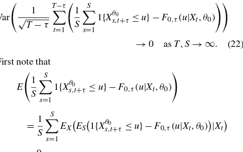
We now show that the first term on the right side of (21) is
oP(1), uniformly in u. Given that 1{Xt≤v} is either 0 or 1,
it suffices to show that √1 T−τ
equality, it thus suffices to show that
Var
whereEX denotes expectation with respect to the probability
law governing the sample, and ES denotes expectation with
respect to the probability law governing the simulated ran-domness, conditional on the sample. Hereafter, let φs(Xt)=
1{Xθ0
Thus, (22) can be written as
1
forT/S→0.This establishes that the first term on the right side of (21) isoP(1),pointwise inu.Uniformity inufollows from
the stochastic equicontinuity of 1{Xθ0
s,t+τ≤u} −F0,τ(u|Xt, θ0).