Full Terms & Conditions of access and use can be found at
http://www.tandfonline.com/action/journalInformation?journalCode=ubes20 Download by: [Universitas Maritim Raja Ali Haji], [UNIVERSITAS MARITIM RAJA ALI HAJI
TANJUNGPINANG, KEPULAUAN RIAU] Date: 11 January 2016, At: 20:38
Journal of Business & Economic Statistics
ISSN: 0735-0015 (Print) 1537-2707 (Online) Journal homepage: http://www.tandfonline.com/loi/ubes20
Principal Volatility Component Analysis
Yu-Pin Hu & Ruey S. Tsay
To cite this article: Yu-Pin Hu & Ruey S. Tsay (2014) Principal Volatility Component Analysis,
Journal of Business & Economic Statistics, 32:2, 153-164, DOI: 10.1080/07350015.2013.818006
To link to this article: http://dx.doi.org/10.1080/07350015.2013.818006
Accepted author version posted online: 12 Jul 2013.
Submit your article to this journal
Article views: 1082
View related articles
View Crossmark data
Principal Volatility Component Analysis
Yu-Pin H
UDepartment of International Business Studies, National Chi Nan University, Taiwan ([email protected])
Ruey S. T
SAYBooth School of Business, University of Chicago, Chicago, IL 60637 ([email protected])
Many empirical time series such as asset returns and traffic data exhibit the characteristic of time-varying conditional covariances, known as volatility or conditional heteroscedasticity. Modeling multi-variate volatility, however, encounters several difficulties, including the curse of dimensionality. Dimension reduction can be useful and is often necessary. The goal of this article is to extend the idea of principal component analysis to principal volatility component (PVC) analysis. We define a cumulative generalized kurtosis matrix to summarize the volatility dependence of multivariate time series. Spectral analysis of this generalized kurtosis matrix is used to define PVCs. We consider a sample estimate of the generalized kurtosis matrix and propose test statistics for detecting linear combinations that do not have conditional heteroscedasticity. For application, we applied the proposed analysis to weekly log returns of seven ex-change rates against U.S. dollar from 2000 to 2011 and found a linear combination among the exex-change rates that has no conditional heteroscedasticity.
KEY WORDS: Common volatility component; Conditional heteroscedasticity; Foreign exchange rate; Generalized covariance matrix; Generalized kurtosis matrix; Principal component analysis.
1. INTRODUCTION
Many empirical time series show the feature of time-varying conditional variance. In economics and finance, this feature is called the conditional heteroscedasticity or volatility. Proper handling of volatility is important in many applications, espe-cially in multivariate setting. For instance, volatility can be used to provide proper interval predictions and to improve density forecasts. In finance, accurate prediction of the conditional co-variance matrix can be used to construct suitable investment portfolios. The commonly used global minimum variance port-folio depends critically on the estimation of volatility matrix of multiple assets. There are indeed many studies concerning sta-tistical models for multivariate volatility; see Bauwens, Laurent, and Rombouts (2006) and the references therein.
Empirical study of multivariate volatility, however, encoun-ters two major difficulties. The first difficulty is the curse of dimensionality. For a k-dimensional time series, there are
k(k+1)/2 conditional variance and covariance processes. Mod-eling the volatility matrix of the components of the S&P 100 index would require analyzing 5050 processes simultaneously. The second difficulty is to maintain the positive definiteness of the estimated volatility matrices. This is not a trivial task when kis large. Many methods have been proposed in the literature to partially overcome these difficulties. See, for instance, Tsay (2010, chap. 10) for a brief discussion of those methods.
An approach to simplify multivariate volatility modeling is di-mension reduction. This is related to the idea of common factors in econometric modeling in which the number of common fac-tors is much smaller than the number of time series. Dimension reduction in volatility modeling is possible provided that there exist some common volatility components in the series under study. With a small number of common volatility components, one can find linear combinations of the time series that have no conditional heteroscedasticity. This idea is similar to that of
the principal component analysis (PCA) in which an eigenvalue close to zero implies the existence of a stable linear combination between the variables. In particular, a zero eigenvalue leads to an exact linear relationship and, hence, the dimension can be reduced.
The goal of this article is to generalize the idea of PCA to principal volatility component (PVC) analysis. The traditional PCA, developed mainly for independent observations, decom-poses ak-dimensional random vector intokcontemporaneously uncorrelated components according to the amount of variability explained by these components. Mathematically, PCA performs the spectral decomposition of the covariance matrix of the ran-dom vector under study. Therefore, our first step in the gener-alization is to define a cumulative generalized kurtosis matrix for multivariate volatility. This matrix summarizes the linear dynamic dependence of volatilities. Spectral decomposition of the proposed cumulative generalized kurtosis matrix enables us to define PVCs. We call such a decomposition the PVC analysis and apply the proposed analysis to detect linear combinations of multiple time series that have no conditional heteroscedasticity. This is equivalent to using the proposed PVC analysis to iden-tify common volatility factors. We also propose a test statistic to verify that a detected linear combination indeed does not have conditional heteroscedasticity. Common volatility components were studied by Engle and Susmel (1993) who used a pairwise procedure.
The proposed PVC analysis is different from applying the traditional PCA to a vector of asset returns, because PCA only produces zero contemporaneous correlations. In other words, PCA overlooks the dynamic dependence between the volatility
© 2014American Statistical Association Journal of Business & Economic Statistics April 2014, Vol. 32, No. 2 DOI:10.1080/07350015.2013.818006
153
processes. The proposed analysis, on the other hand, focuses on the dynamic dependence of the volatility. It is concerned with the fourth moment, both serial and cross-sectional, of a vector time series. Details are given in Section3.
The article is organized as follows. In Section 2, we state clearly the conditional heteroscedasticity considered in this ar-ticle and define the proposed cumulative generalized kurtosis matrix of ak-dimensional time series. Some properties of the proposed matrix are given. In Section3, we introduce PVCs and discuss their properties. Section4considers sample estimate of the cumulative generalized kurtosis matrix and sample PVC. It also proposes a test statistic for verifying that an estimated linear combination of the observed time series has constant conditional variance. Simulations are used to demonstrate the performance of the proposed PVC analysis and the test statistic in finite sam-ples. Section5considers an application of the proposed PVC analysis using weekly log returns of seven foreign exchange rates, and Section6concludes. All proofs are in the Appendix.
2. CONDITIONAL HETEROSCEDASTICITY AND GENERALIZED KURTOSIS MATRIX
Let yt =(y1t, . . . , ykt)′ be a k-dimensional weakly
sta-tionary time series with finite fourth moment. Let Ft−1 = σ{yt−1,yt−2, . . .}, denoting the information available at time t−1. Since we focus on volatility, we assumeE(yt|Ft−1)=
0. The volatility matrix t of yt is then defined as t ≡
cov(yt|Ft−1)=E(yty′t|Ft−1). We assume that the volatility ma-trix can be written as
vec(t)=c0+ ∞
i=1
Civec(yt−iy′t−i), (1)
where vec(M) denotes the column-stacking vector of the matrix M,c0is ak2-dimensional positive constant vector, andCi are
k2
×k2constant matrices fori >0. The matricesC
iand vector
c0 satisfy certain conditions to ensure thatt is positive
defi-nite for allt. The Baba–Engle–Kraft–Kroner (BEKK) model of Engle and Kroner (1995) can be written in the form of Equation (1) via repeated substitutions. From Equation (1), the processyt
has conditional heteroscedasticity if and only ifCi=0for some
i >0. For multivariate autoregressive conditional heteroscedas-tic (ARCH) models, the summation in Equation (1) is truncated at a finite lag. In this article, we say that a vector time series yt
has ARCH effects or conditional heteroscedasticity if Ci =0
for somei >0.
From Equation (1), the existence of ARCH effects in yt
im-plies that yty′t is correlated with yt−iy′t−i for somei >0. This
motivates us to define the lag-ℓgeneralized kurtosis matrixγℓ
of yt as
γℓ=
k
i=1
k
j=i
cov2(yty′t, xij,t−ℓ)≡ k
i=1
k
j=i
γℓ,ijγ′ℓ,ij,
forℓ≥0, (2)
wherexij,t−ℓis a function ofyi,t−ℓyj,t−ℓfor 1≤i, j≤k,
γℓ,ij=cov(yty′t, xij,t−ℓ)=E[(yty′t−)(xij,t−ℓ−E(xij,t))],
(3)
and=E(yty′t) is the unconditional covariance matrix of yt.
The matrixγℓ,ijof Equation (3) is called a generalized covari-ance matrix in the statistical literature, for example, Li (1992). It is ak×ksymmetric matrix, but might be negative definite. However, its square matrix, which is equivalent toγℓ,ij(γℓ,ij)′, is semipositive definite. This justifies the use of square in Equa-tion (2). From the definiEqua-tion, the lag-ℓgeneralized kurtosis ma-trixγℓis symmetric and semipositive definite, because it is the
sum ofk(k+1)/2 symmetric and semipositive definite matri-ces. An important property ofγℓ is thatγℓ=0if and only if
yty′tis not correlated withyi,t−ℓyj,t−ℓfor alliandj.
For a given positive integerm, we define the cumulative gen-eralized kurtosis matrix as
Ŵm= m
ℓ=1
γℓ. (4)
This cumulative matrix is symmetric and semipositive definite, and we use it to measure the ARCH(m) effects in yt. For the
general multivariate GARCH-type models, we consider
Ŵ∞=
∞
ℓ=1
γℓ, (5)
which is assumed to exist. We refer toŴ∞as the cumulative generalized kurtosis matrix of yt.Ŵ∞ is also symmetric and semipositive definite.
2.1 Properties of Generalized Kurtosis Matrix
The idea of generalized covariance matrix cov(yty′t, xt),
where xt is a scalar random variable, has been used in the
statistical literature. See, for instance, Li (1992). To the best of our knowledge, the concept has not been used in the time series analysis. In this section, we discuss some properties of the generalized kurtosis matrix in Equation (5) that are relevant to our study.
Let M be a k×k nontrivial linear transformation matrix so that zt =M′yt is a transformed series. For asset returns,
columns of M may represent, after normalization, investment portfolios. Letxt−1be a scalar function of elements ofFt−1, for example,xt−1=yi,t−hyj,t−h for someh >0. It is easy to see
that the following lemma holds.
Lemma 1. For a constant k×k matrix M, let zt =
M′yt. Then, cov(ztz′t, xt−1) = cov(M′yty′tM, xt−1) = M′cov(yty′t, xt−1)M.
Letmv =(m1v, . . . , mkv)′be thevth column ofM. Ifzvt =
m′
vyt is a linear combination of yt that has no ARCH effects,
then we haveE(z2
vt|Ft−1)=cv2, which is a constant. This implies
that z2
vt is not correlated with yi,t−ℓyj,t−ℓ for ℓ >0 and 1≤
i, j≤k. In other words, cov(z2
vt, yi,t−ℓyj,t−ℓ)=0 forℓ >0 and
1≤i≤j ≤k. Using Lemma 1, we see thatγℓ,ijis singular for all ℓand 1≤i≤j ≤k and, hence, γℓ is singular for all ℓ. Consequently,Ŵ∞is also singular.
On the other hand, assume that Ŵ∞ is singular and mv is
in its null space. That is,Ŵ∞mv =0. Sinceγℓis semipositive
definite, we havem′vγℓmv =0 for allℓ. This in turn shows that
m′vγ
2
ℓ,ijmv =0 for allℓ >0 and 1≤i≤j ≤k. Consequently,
by the symmetry of γℓ,ij, we have (γℓ,ijmv)′(γℓ,ijmv) = 0.
This implies thatγℓ,ijmv=0for allℓ >0 and 1≤i≤j ≤k.
Again, using Lemma 1, we see thatz2
vt is not correlated with
yi,t−ℓyj,t−ℓ for ℓ >0 and 1≤i≤j ≤k, where zvt = m′vyt.
This implies thatE(z2
vt|Ft−1) is not time varying. In other words, zvt does not have conditional heteroscedasticity. The above
dis-cussion shows that an eigenvector ofŴ∞associated with a zero eigenvalue gives rise to a linear combination of yt that has no
ARCH effect. We summarize the above result into a theorem.
Theorem 1. Consider a weakly stationary process yt with
finite fourth moment and satisfying Equation (1). LetŴ∞be the cumulative generalized kurtosis matrix defined in Equation (5), where xij,t−ℓ=yi,t−ℓyj,t−ℓ in Equation (3). Then, there exist
k−mlinearly independent linear combinations ofyt that have
no ARCH effects if and only if rank(Ŵ∞)=m.
3. PRINCIPAL VOLATILITY COMPONENTS
Consider the spectral decomposition of the cumulative gen-eralized kurtosis matrix Ŵ∞, say Ŵ∞M=M, where =
diag{λ2
1≥λ22≥ · · · ≥λ2k} is the diagonal matrix of ordered
eigenvalues andM =[m1, . . . ,mk] is the matrix of
eigenvec-tors. Here, we use the notationλ2vto denote eigenvalues because
Ŵ∞is semipositive definite. We assume that the columnsmvare
normalized withmv =1.
We define thevth PVC of ytaszvt =m′vyt. From the
defini-tion and spectral decomposidefini-tion ofŴ∞, we have ∞
ℓ=1
k
i=1
k
j=i
m′vγ
2
ℓ,ijmv =λ2v, v=1, . . . , k. (6)
Let γℓ,ijmv=wℓ,ij,v. Then, we have ∞ℓ=1
k i=1
k j=i
w′
ℓ,ij,vwℓ,ij,v =λ2v. Using Lemma 1, we have
m′vwℓ,ij,v=m′vγℓ,ijmv=cov
z2vt, xij,t−ℓ
. (7)
This result indicates thatm′
vγℓ,ijmvcan be regarded as a
mea-sure of the dependence of volatility of the portfoliozvt on the
lagged cross-product termxij,t−ℓ. In practice, this quantity can
be negative so that we use squared matrices in Equation (6) to construct a nonnegative dependence measure.
From Equation (6),λ2v summarizes the dependence measure in Equation (7) over all combinations of i andj and over all lags. As such, it can be considered as an approximate measure of volatility dependence of the portfolio zvt. A larger λv is
indicative of a stronger volatility dependence. Therefore, we call zvt the vth PVC. On the other hand, the summation in
Equation (6) distinguishes the PVC from the traditional principal components of yt, which depends on the covariance matrix
alone. The PVC analysis is designed to consider simultaneously volatility dependence at all past lags.
Since Ŵ∞ is semipositive definite, its eigenvectors are or-thogonal provided that the associated eigenvalues are distinct. Consequently, any two PVCs,zvt =m′vyt andzut=m′uyt, are
uncorrelated ifλ2v=λ2u. On the other hand, for PVCzvt
associ-ated with a nonzeroλ2v,z2vt may still be correlated with lagged values ofz2ut. Our limited experience indicates that such corre-lations, if exist, are of smaller magnitudes compared with those of the observedyit2 series.
Like the traditional PCA, an important application of the proposed PVC analysis is to reduce the dimension in volatility modeling. To this end, the number of zero eigenvalues ofŴ∞is
of special interest. By Theorem 1, we have common volatility components if the cumulative generalized kurtosis matrixŴ∞is not of full rank. We explore possible applications of this property in Section5.
4. SAMPLE PRINCIPAL VOLATILITY COMPONENTS
In this section, we consider estimation of the generalized kurtosis matrices and obtain the sample PVCs. We establish some consistency properties of the sample estimate ofŴ∞. Fur-thermore, to verify that a given portfolio does not have ARCH effects, we propose a test statistic and establish its asymptotic distribution.
To simplify the moment restrictions on ytfor making
statisti-cal inference ofŴ∞orŴm, we follow the approach of Matteson
and Tsay (2011) by employing the Huber’s function of the cross-product variableyi,t−ℓyj,t−ℓ:
xij,t−ℓ=
⎧ ⎪ ⎨ ⎪ ⎩
yi,t−ℓyj,t−ℓ if|yi,t−ℓyj,t−ℓ| ≤c2
2c√yi,t−ℓyj,t−ℓ−c2 ifyi,t−ℓyj,t−ℓ> c2
c2
−2c|yi,t−ℓyj,t−ℓ| ifyi,t−ℓyj,t−ℓ<−c2,
(8)
wherecis a prespecified constant.
Note that the necessary part of Theorem 1 continues to hold if we substituteyi,t−ℓyj,t−ℓinŴℓby the Huber’s functionxij,t−ℓ
of Equation (8). The sufficient part of the theorem, however, may not hold. This weakness, however, can be out-weighted by the gain obtained in relaxing the moment conditions needed for the estimation and testing discussed in Theorems 2 and 3. In what follows, we adopt the xij,t−ℓ of Equation (8) to
de-fine the sample generalized kurtosis matrix using Equation (3) and the corresponding cumulative generalized kurtosis matrix. Obviously,xij,t−ℓapproachesyi,t−ℓyj,t−ℓascincreases.
4.1 Estimation
Given the data {r1, . . . ,rn}of a stationary process rt, we
employ the normalized data{y1, . . . ,yn}, where yt =
−1/2 rt
withbeing the sample covariance matrix ofrt. The
normal-ization is taken to increase the numerical stability of estimation because asset returns tend to be small. Let
cov(yty′t, xij,t−ℓ)=
1
n
n
t=ℓ+1
(yty′t−Y¯)(xij,t−ℓ−x¯ij),
where ¯Y and ¯xij are the sample mean of yty′t andxij,t,
respec-tively. This is the sample counterpart of the lag-ℓgeneralized kurtosis matrix with the Huber’s function of the lagged cross-product variable. We estimateŴmby
Ŵm= m
ℓ=1
k
i=1
k
j=i
1−ℓ
n
2
cov2(yty′t, xij,t−ℓ). (9)
Suppose yt is stationary with finite sixth moment and the
as-sumptionA.1in the Appendix holds. Then, for a fixed positive integerm <∞,
Ŵm=Ŵm+Op
1 √
n
.
We estimateŴ∞by
a positive real number depending onn.
Under the regularity conditions used in spectral density esti-mation (Hannan1970), andmn/n→0, mn→ ∞asn→ ∞,
we have
Ŵn=Ŵ∞+Op(an), (11)
whereanis a function ofmnandn. Some guidelines for choosing
mnare as follows: the convergence rate ofŴnof Equation (11)
depends on the minimal mean squared errorE(Ŵn−Ŵ∞)2.
For a specific smoothing functionw∗(.), we can selectmn care-fully to achieve the minimal mean squared error. For exam-ple, ifw⋆ is the Bartlett’s smoothing function, the best choice
of mn is mn=n1/3 such that an=n−1/3, and if w⋆ is the
Daniell’s smoothing function, one can choosemn=n1/5such
thatan=n−2/5. See Hannan (1970) for details.
For simplicity, we use the estimateŴmof Equation (9) in our
applications. We check the stability of the results with several choices ofm. For a given estimateŴm, we perform eigenvalue–
eigenvector analysis to obtain the sample PVCs. Specifically, the vth sample volatility component is ˆzvt =m′vyt =m′v
−1/2 rt,
wheremvis the normalized eigenvector of thevth eigenvalue of
Ŵm. Finally, we perform hypothesis testing to check the ARCH
dependence of the sample PVCs at all lags, not just the firstm lags.
4.2 Testing
An important application of the proposed PVC analysis is dimension reduction. Here dimension reduction means finding linear combinations of yt that have no ARCH effects. LetM1 be a k×s matrix consisting of eigenvectors associated with thessmallest eigenvalues of theŴm (orŴ∞) matrix. In other words,M1gives rise to the (k−s+1)th to thekth PVCs ofyt.
Our goal here is to consider test statistics for verifying that the transformed series ˆet =M′1ytindeed has no ARCH effects.
Many data-generating processes (DGPs) of yt can lead to
linear combinations ofytthat have no ARCH effects. Consider,
for instance, the case of common volatility components, which is the focus of our application in Section5. Assume that
yt =H ft+ǫt, (12)
where H is a k×r real-valued matrix of rank r, ft =
(f1t, . . . , frt)′ consists of r independent conditional
het-eroscedastic processes,{ǫt}is a sequence of independent and
identically distributed random vectors with mean zero and con-stant positive-definite covariance matrix ǫ, and ǫt is
inde-pendent of ft. Based on the definition of Equation (1), each
volatility component var(fit|Ft−1) is a nontrivial function of el-ements of{yt−jy′t−j|j >0}. For this particular DGP, ifr < k,
then the volatility of ytis driven by ther-dimensional common
volatility components in ft. LetM1be ak×(k−r) real-valued matrix such thatM′
1H=0. Letet =M′1yt. It is easy to see that
et =M′1ǫtand, hence, it has no ARCH effects.
There are several tests available in the literature to check for multivariate ARCH effects. In this section, we generalize the results of Ling and Li (1997), Duchesne and Lalancette (2003), Duchesne and Roy (2004), and Hong (1996) to derive two test statistics that are applicable to the PVC analysis. The generalization is mainly to deal with the fact that M1 is an estimate and the dimensionsof ˆetcould be smaller thank. We
establish the limiting distributions of the proposed test statistics. All proofs are given in the Appendix.
4.2.1 Ling–Li Test Statistic. Following Ling and Li (1997), we define
sample covariance matrix of ˆetandyt. Furthermore, let
ǫt =
positive integerd, consider the hypothesis testingH0:ρ1,s=
ρ2,s= · · · =ρd,s=0 versusHa :ρi,s =0 for some 1≤i≤d,
whereρj,sis the correlation betweenǫt andxt−j. The Ling–Li
test statistic for the hypotheses is
Td,s =nR′d,s
diagonal matrix. In this case,Td,s reduces to the original Ling
and Li test statistic.
Theorem 2. Suppose that yt is ak-dimensional weakly
sta-tionary time series with ARCH dynamic given in Equation (1). Assume that the sixth moment of yt exists and M1 is the full-rank transformation matrix such that et =M′1yt has no
ARCH effects. Under the AssumptionA.1in the Appendix, if √
nan2→0, whereanis the convergence rate of M1 toM1 as given in Equation (11), then
√
n−d,s1/2Rd,s→d N(0,Id×d), and
Td,s=nR′d,s
−1
d,sRd,s→d χd2,
where→d denotes convergence in distribution.
4.2.2 Generalized Test Statistic. The Td,s statistic is
de-signed to detect the serial volatility dependence in the firstd lags. In empirical applications, one would prefer a test statistic that can account for volatility dependence in all past lags. To this end, we adopt the idea of Hong (1996) to derive a generalized Ling–Li test statistic. The generalized test statistic is defined as
Gpn,s=
nnj−=11w2(j/pn) ˆρ2j,s−Mn(w)
[2Vn(w)]1/2
, (15)
where Mn(w)=
n−1
j=1(1−j/n)w2(j/pn), Vn(w)=
n−2
j=1(1− j/n)[1−(j+1)/n]w4(j/pn), =1+2
∞
h=1cov 2(x
t, xt−h),
pn is a function of n such that pn→ ∞ and pn/n→0 as
n→ ∞, andw(.) is a symmetric kernel function.
If yt is a k-dimensional process of independent and
iden-tically distributed random variables, then s=k. In this case,
Gpn,s reduces to the Hong’s statistic in which=1 because
cov2(x
t, xt−h)=0 for allh >0. In this sense,is used to
ad-just for the ARCH effects in theyt series. This quantity can be
estimated by a smoothing method as
=1+2
n−1
h=1
k(h/sn)cov2( ˆxt,xˆt−h), (16)
wherek(.) is a kernel function satisfying some regularity con-ditions such that ∗=1+2nh−=11k(h/sn)cov2(xt, xt−h) is a
consistent estimate of and sn is a function of n such that
sn→ ∞andsn/n→0 asn→ ∞. In this article, we use the
Daniell functiong(x)=sin(π x)/(π x) for bothw(x) andk(x).
Theorem 3. Suppose that yt is ak-dimensional weakly
sta-tionary process with ARCH effects governed by Equation (1) and has finite sixth moment. Let M1 be a constant full-rank k×stransformation matrix such thatet =M′1ythas no ARCH
effects. Assume that M1 is a consistent estimate of M1 and ˆ
et =M′1yt. Under the Assumptions A.1 and A.2 of the
Ap-pendix, if pn→ ∞,pn/n→0, na4
n
√p
n →0, andpna
2
n→0 as
n→ ∞, thenGpn,s→d N(0,1), whereGpn,sis the test
statis-tic in Equation (15) andanis given in Equation (11).
4.2.3 Testing for ARCH Effects. For a given dataset, let
Ŵm be the sample estimate of the cumulative generalized
kur-tosis matrix. Further, let M = [m1, . . . ,mk] be the matrix
of standardized eigenvectors such thatŴmmv =λ2vmv, where
λ2 1≥λ
2
2≥ · · · ≥λ 2
kare the eigenvalues. Since zero eigenvalues
ofŴmgive rise to components without ARCH effects, we
con-sider the following test procedure to detect linear combinations of yt that have no ARCH effects. Letsbe the number of
lin-ear combinations of yt that have no ARCH effects. LetM1= [mk, . . . ,mk−s+1] be thek×s matrix consisting of the lasts columns of M, that is, consisting of the standardized eigen-vectors ofŴmcorresponding to thessmallest eigenvalues. Let
ˆ
et =M′1yt be thes-dimensional transformed process
consist-ing of the last s PVC series of yt. We apply the generalized
Ling–Li test statistic of Theorem 3 to test the null hypothesis that ˆet has no ARCH effects. In practice, we perform the test
for s=1, . . . , k. If the null hypothesisH0:s=s∗ is not re-jected, but the null hypothesisH0:s=s∗+1 is rejected, then we have s∗ linear combinations of yt that have no ARCH
ef-fects. In other words, we test sequentially the hypothesis that the smallestseigenvalues ofŴmare zero.
4.3 Simulation Study
We use simulations to study the finite-sample performance of the proposed PVC analysis and the test statistics Td,s and
Gpn,sof Equations (14) and (15). In particular, we investigate
the effects of the choices of tuning parameters pn andsn on
the behavior of Gpn,s and the accuracy of the estimation of
the no-ARCH portfolio. The DGP employed is the model in Equation (12) with ytbeing a five-dimensional series (i.e.,k=
5) and ft =(f1t, . . . , f4t)′such thatfit =σiteit, where
σ12t =1+0.9f12,t−1, σ22t =2+0.8f22,t−1,
σ32t =3+0.7f32,t−1, σ42t =1+0.95f42,t−1,
and {eit} are sequences of independent and identically
dis-tributed (iid) standard normal random variables and {eit}and
{ej t}are independent fori=j. We understood that these four
ARCH(1) models do not satisfy the moment condition of The-orems 2 and 3. However, we expect the proposed PVC analysis continues to work reasonably well in finite samples for these four processes similar to the fact that the traditional PCA analy-sis does to the unit-root nonstationary time series; see Box and Tiao (1977). The loading matrix is H=[h1,h2,h3,h4] with h1 =(1,1,1,1,1)′,h2=(1,0,0,0,0)′,h3=(0,1,0,−1,0)′, andh4 =(0,0,−1,0,1)′, and the noise term{ǫt}is a sequence
of iid standard multivariate normal random vectors. In this par-ticular instance, M1=(0,−1,1,−1,1)′ gives rise to the no-ARCH portfolio. Letm1be the normalized eigenvector corre-sponding to the smallest eigenvalue of theŴm matrix. Under
the proposed PVC analysis,m1is a consistent estimate ofM1. To measure the performance of the proposed PVC analysis, we consider the following two statistics
R1= | m′
1H(H′H)−1H′m1| |m′
1m1|
, R2=cor2(m1′yt,M′1yt),
(17)
and expectR1≈0 andR2≈1.
In the simulation, we considerd=pn∈ {5,10,20,40},sn∈
{5,10,20}, and sample size ranging from 250 to 2000. For a given sample size, we used the DGP to generate 10,000 datasets ofytand applied the proposed PVC analysis and the test
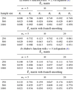
Table 1. Summary statistics of the proposed principal volatility component analysis for a five-dimensional series with four common
ARCH(1) components
(a) Huber’s function withc=2.5 in Equation (8)
Ŵmmatrix
m=5 10 20
Sample size R1 R2 R1 R2 R1 R2
250 0.086 0.768 0.089 0.749 0.092 0.746
500 0.023 0.906 0.028 0.894 0.029 0.893
1000 0.006 0.965 0.006 0.961 0.007 0.956
Ŵnmatrix with Daniell smoothing
mn=5 10 20
250 0.093 0.752 0.123 0.702 0.135 0.681
500 0.029 0.903 0.043 0.871 0.062 0.839
1000 0.007 0.966 0.013 0.951 0.027 0.931
(b) Huber’s function withc=5 in Equation (8)
Ŵmmatrix
m=5 10 20
250 0.100 0.729 0.110 0.714 0.111 0.710
500 0.039 0.868 0.043 0.857 0.047 0.850
1000 0.013 0.944 0.013 0.945 0.016 0.930
Ŵnmatrix with Daniell smoothing
mn=5 10 20
250 0.122 0.701 0.159 0.647 0.174 0.625
500 0.050 0.855 0.077 0.809 0.102 0.770
1000 0.021 0.934 0.030 0.921 0.051 0.879
NOTES: The performance measuresR1andR2of Equation (17) are calculated using 10,000
iterations. For theŴmmatrix, we usem=5, 10, and 20. For theŴnmatrix, we use the
Daniell smoothing method withmn=5, 10, and 20. The expected values ofR1andR2are
0 and 1, respectively.
statisticsTd,s andGpn,sto the data.Table 1reports the
perfor-mance of the proposed PVC analysis via the measuresR1andR2 of Equation (17). Here, we consider different choices ofmfor the cumulative generalized kurtosis matrixŴmof Equation (9)
and different choices ofmnin estimatingŴnusing the Daniell
smoothing method. For the Huber’s function in Equation (8), we usec=2.5 andc=5. The results show that the proposed PVC analysis works well when the sample sizen≥500. Fur-thermore, the PVC analysis usingŴm outperforms that using
Ŵn. In general, results of the simulation support the use ofŴm
withc=2.5 andm=5 or 10 for the PVC analysis.
Based on the results ofTable 1, we use Ŵ10 withc= 2.5 in the Huber’s function in Equation (8) in our further study. Table 2summarizes the size and power of the Ling–Li statistic
Td,sof Equation (14). From the table, it is seen that the Ling–Li
statistic does not fare well in the presence of ARCH effects. However, the test statistic works reasonably well when the sam-ple size is large, say 2000. Since we havek=5 series andr=4 common volatility factors, the size and power of the test statistic are obtained from the hypothesess=1 and 2, respectively.
Table 3summarizes the empirical size and power of the mod-ified test statisticGpn,s of Equation (15) over the 10,000
iter-ations for various choices ofpnandsn. Again, the same DGP
is used and the size and power are for the case ofs=1 and 2, respectively. We also report the adjusted term, but find that it is far away from 1, indicating strong ARCH effects in the data.
5. APPLICATION
In this section, we apply the proposed PVC analysis and the generalized Ling–Li test statistic to the weekly log returns of seven foreign exchange rates against U.S. Dollar from March 2000 to October 2011. Our analysis shows that there exists a linear combination in the log returns that has no conditional heteroscedasticity. In other words, we found common volatility components in the exchange markets in the period from March 2000 to October 2011.
Consider the exchange rates of British Pound (x1t),
Norwe-gian Kroner (x2t), Swedish Kroner (x3t), Swiss Franc (x4t),
Canadian Dollar (x5t), Singapore Dollar (x6t), and Australian
Dollar (x7t) against U.S. Dollar from March 22, 2000 to
Octo-ber 26, 2011. We use weekly average to compute the log returns. That is, definert =ln(xt)−ln(xt−1), wherextis the vector of
Table 2. Summary statistics of the Ling–Li test statisticTd,nof Equation (14) for a five-dimensional series with four common ARCH components
Type I: 0.05 Type I: 0.10
Sample size d=5 10 20 40 5 10 20 40
250 0.019 0.022 0.047 0.065 0.042 0.041 0.074 0.104
500 0.033 0.039 0.059 0.072 0.062 0.069 0.095 0.114
750 0.039 0.051 0.062 0.078 0.074 0.084 0.098 0.122
1000 0.049 0.052 0.068 0.079 0.088 0.087 0.109 0.125
2000 0.048 0.054 0.077 0.071 0.088 0.096 0.114 0.123
Power
250 0.057 0.034 0.059 0.075 0.101 0.064 0.090 0.113
500 0.245 0.159 0.134 0.135 0.330 0.226 0.189 0.182
750 0.461 0.338 0.252 0.207 0.552 0.424 0.332 0.267
1000 0.654 0.519 0.412 0.302 0.728 0.606 0.491 0.371
2000 0.947 0.896 0.805 0.674 0.965 0.928 0.855 0.736
NOTE: The results are based onŴ10withc=2.5 for the Huber’s function in Equations (8) and (13), and 10,000 iterations.
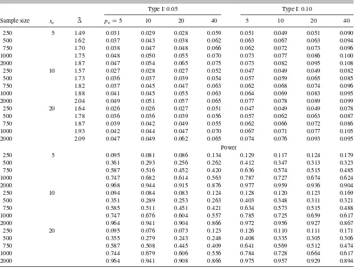
Table 3. Summary statistics of the modified test statisticGpn,sof Equation (15) for a five-dimensional series with four common ARCH components
Type I: 0.05 Type I: 0.10
Sample size sn pn=5 10 20 40 5 10 20 40
250 5 1.49 0.031 0.029 0.028 0.059 0.051 0.049 0.051 0.090
500 1.62 0.037 0.043 0.038 0.062 0.063 0.067 0.063 0.094
750 1.70 0.038 0.047 0.048 0.066 0.062 0.072 0.073 0.096
1000 1.75 0.048 0.050 0.055 0.070 0.073 0.077 0.086 0.100
2000 1.87 0.047 0.054 0.065 0.075 0.073 0.082 0.095 0.108
250 10 1.57 0.027 0.028 0.027 0.052 0.047 0.049 0.049 0.082
500 1.73 0.036 0.037 0.039 0.054 0.057 0.059 0.065 0.085
750 1.82 0.037 0.045 0.047 0.063 0.062 0.068 0.074 0.096
1000 1.88 0.041 0.045 0.055 0.063 0.064 0.069 0.083 0.095
2000 2.04 0.049 0.051 0.057 0.065 0.077 0.078 0.089 0.099
250 20 1.64 0.026 0.026 0.027 0.051 0.047 0.049 0.049 0.078
500 1.78 0.036 0.036 0.039 0.056 0.057 0.062 0.063 0.087
750 1.87 0.039 0.042 0.049 0.055 0.062 0.066 0.072 0.086
1000 1.93 0.042 0.044 0.047 0.070 0.067 0.071 0.077 0.105
2000 2.09 0.047 0.049 0.062 0.065 0.074 0.076 0.093 0.095
Power
250 5 0.095 0.081 0.086 0.134 0.129 0.117 0.124 0.179
500 0.361 0.293 0.256 0.262 0.412 0.347 0.313 0.323
750 0.587 0.516 0.452 0.420 0.636 0.574 0.515 0.485
1000 0.747 0.682 0.614 0.563 0.787 0.727 0.674 0.624
2000 0.968 0.944 0.915 0.876 0.977 0.959 0.936 0.904
250 10 0.094 0.084 0.083 0.124 0.128 0.120 0.123 0.169
500 0.351 0.289 0.253 0.263 0.403 0.348 0.311 0.321
750 0.585 0.511 0.451 0.421 0.634 0.573 0.515 0.488
1000 0.747 0.676 0.604 0.557 0.785 0.725 0.659 0.617
2000 0.964 0.941 0.904 0.866 0.972 0.956 0.927 0.867
250 20 0.095 0.076 0.073 0.123 0.126 0.110 0.111 0.171
500 0.355 0.279 0.243 0.248 0.408 0.335 0.305 0.306
750 0.587 0.508 0.445 0.409 0.641 0.569 0.512 0.474
1000 0.744 0.679 0.606 0.556 0.784 0.728 0.664 0.617
2000 0.964 0.941 0.908 0.866 0.975 0.957 0.929 0.894
NOTE: We use 10,000 iterations andŴ10withc=2.5 for the Huber’s function in Equations (8) and (13), wheresnandare given in Equation (16).
weekly averages of daily exchange rates of weekt. This results in seven return series each with 605 observations. We also used weekly log returns from Wednesday to Wednesday and obtained similar results.
Preliminary analysis shows that there are some serial and cross-correlations in the return seriesrt. We employ vector
au-toregressive (VAR) models with Akaike information criterion to handle the serial correlations of the returns. It turns out a VAR(5) model is sufficient to remove the serial and cross-correlations in rt. Consequently, our PVC analysis is carried out on the
residualsǫt of a VAR(5) model forrt.Table 4provides some
summary statistics of the residual seriesǫt. From the table, we
see that each residual series has no serial correlations, but has strong ARCH effects; see the Ljung–Box statistics ofǫt and
its squared series. In fact,p-values of the Ljung–Box statistics
Q(10) for the squared residuals are all close to zero, indicating strong ARCH effects in the seven residual series.
We employ the sample estimateŴmof the cumulative
gen-eralized kurtosis matrix of ǫt to perform the proposed PVC
analysis usingc=2.5 for Huber’s function in Equation (8) and
m∈ {5,10,15,20}. We also employŴnwith Daniell
smooth-ing with mn=5,10,15,20. All results of the PVC analysis
are similar. Consider, for instance, the test results summa-rized in Table 5. Using c=2.5 in the Huber’s function of Equation (13), we apply the proposed generalized Ling–Li test statistic to search for linear combinations of the returns that have no ARCH effects. The testing results based onŴ10are given in Table 5(a) for differentpnvalues. Parts (b)–(d) ofTable 5show
the test results forŴmwithm=5, 15, and 20, respectively. Parts
(e) and (f) of the table give the test results usingŴnwithmn=
10 and 5, respectively. All test results are in agreement with that based onŴ10in Part (a). Therefore, this particular example demonstrates that the proposed PVC analysis is not sensitive to the choice ofmso long asm≥5. In what follows, we focus on the results ofŴ10.
FromTable 5, we see that there exists a portfolio of the ex-change rates that has no ARCH effects, and this conclusion does not depend on the choice ofpn of the test statistic. Our
analysis thus indicates that there are common volatility compo-nents in the weekly log returns of the seven exchange rates be-tween March 2000 and October 2011. The resulting eigenvalues and standardized eigenvectors ofŴ10 are given inTable 6. The
Table 4. Summary statistics of the residuals of a VAR(5) model for weekly log returns of seven currencies versus U.S. dollar
Stat GBP NOK SEK CHF CAD SGD AUD
s.e. 0.0101 0.0131 0.0131 0.0120 0.0105 0.0053 0.0144
Skewness 0.4681 0.5578 0.4581 0.3369 0.4765 0.5866 0.9295
Kurtosis 0.7419 0.5970 0.8454 1.3008 1.2973 1.1980 2.2019
Q(10,ǫt) 5.68(.8) 2.80(1.) 7.84(.6) 9.58(.5) 4.46(.9) 5.86(.8) 11.42(.3)
Q(10,ǫ2
t) 74.73 90.87 42.95 56.09 235.3 41.46 93.04
NOTES: The seven currencies are British pound (GBP), Norwegian kroner (NOK), Swedish kroner (SEK), Swiss franc (CHF), Canadian dollar (CAD), Singapore dollar (SGD), and Australian dollar (AUD). The sample period is from March 29, 2000 to October 26, 2011. Values in parentheses denote approximatep-values andQ(.) denotes the Ljung–Box test statistics for no serial correlations.
eigenvectors are used to obtain the PVCs of the weekly log re-turns of seven exchange rates. The loadings of the portfolio with no ARCH effects are given in Column 1 ofTable 6, whereas those for the common volatility components are given in the last six columns.
To gain further insight into PVCs, we perform some univariate analyses of the sample PVCs. Letej t=m′jǫt be thejth PVC
series. Our test results show thate7thas no ARCH effects, but the
remaining six PVCs have ARCH effects.Table 7shows some results of Ljung–Box test for serial correlations and ARCH
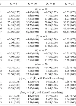
Table 5. Results of generalized Ling–Li tests for no ARCH effects of principal volatility components for weekly log returns of seven
exchange rates from March 29, 2000 to October 26, 2011
s pn=5 pn=10 pn=15 pn=20
(a)m=10
1 −0.74(0.77) −1.02(0.85) −0.73(0.77) −0.53(0.70)
2 3.95(0.00) 4.65(0.00) 4.78(0.00) 5.51(0.00)
3 11.55(0.00) 13.31(0.00) 13.40(0.00) 14.23(0.00)
4 27.45(0.00) 30.03(0.00) 30.06(0.00) 30.93(0.00)
5 34.18(0.00) 37.70(0.00) 36.83(0.00) 36.09(0.00)
6 43.91(0.00) 48.17(0.00) 48.11(0.00) 47.40(0.00)
7 57.06(0.00) 62.36(0.00) 64.02(0.00) 64.84(0.00)
(b)m=5
1 −0.76(0.77) −1.08(0.86) −0.83(0.79) −0.63(0.73)
2 2.36(0.01) 3.78(0.00) 5.21(0.00) 7.36(0.00)
3 9.99(0.00) 12.24(0.00) 13.05(0.00) 14.43(0.00)
(c)m=15
1 −0.75(0.77) −1.03(0.85) −0.78(0.78) −0.61(0.73)
2 4.90(0.00) 4.98(0.00) 4.43(0.00) 4.06(0.00)
3 12.41(0.00) 13.52(0.00) 13.27(0.00) 13.66(0.00)
(d)m=20
1 −0.74(0.77) −1.01(0.85) −0.79(0.79) −0.63(0.73)
2 5.23(0.00) 5.18(0.00) 4.54(0.00) 4.06(0.00)
3 21.70(0.00) 22.54(0.00) 21.30(0.00) 19.99(0.00)
(e)mn=10 (Ŵnwith Daniell smoothing)
1 −0.78(0.78) −1.10(0.87) −0.88(0.81) −0.68(0.75)
2 2.45(0.01) 3.85(0.00) 5.08(0.00) 7.16(0.00)
3 10.29(0.00) 13.42(0.00) 14.65(0.00) 16.61(0.00)
(f)mn=5 (Ŵnwith Daniell smoothing)
1 −0.71(0.76) −1.02(0.85) −0.77(0.78) −0.57(0.72)
2 2.37(0.01) 4.24(0.00) 6.42(0.00) 9.04(0.00)
3 8.81(0.00) 13.59(0.00) 16.85(0.00) 19.03(0.00)
NOTES: In the table,mdenotes the number of lags used to estimateŴm,pndenotes the
window length used in the generalized testGpn,sof Equation (15), andsis the number of principal volatility components used. Also, number in parentheses denotesp-value.
effects for selected PVCs. The table also includes parameter estimates and their standard errors of fitting an ARCH(5) model to the components. From the table, we observe that (a) the PVCs have no serial correlations based on the Ljung–Box statistics
Q(10) and (b) as expected, PVCe7t has no ARCH effects but
e6tande1tdo. The ARCH effects ofe1tande6tare confirmed by
both the Ljung–Box statisticsQ(10) of the squared series and the parameter estimates of an ARCH(5) model.
FromTable 6, the no-ARCH portfolio can be written, to a rough approximation, as
e7t ≈0.2(GBP+NOK+SEK+CHF+AUD)
−0.6(CAD+SGD),
showing that the no-ARCH portfolio basically consists of the exchange rates of European countries and Australian (against U.S. Dollar) versus those of Canada and Singapore (against U.S. Dollar). It is interesting to see that the sample stan-dard errors of the log returns of the seven exchange rates are 0.0114(GBP), 0.0141(NOK), 0.0142(SEK), 0.0130(CHF), 0.0114(CAD), 0.0059(SGD), and 0.0158(AUD), respectively. The portfolio appears to be a weighted difference between equally weighted sum of the five more variable exchange rates and that of the two less variable exchange rates. The existence of such a portfolio is plausible as carry trade and exchange hedging might be based on the variabilities of the exchange rates.
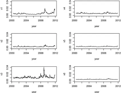
Finally, some discussion is in order.Figure 1shows the time plots of the volatility series for the first six PVCs. The volatility series are obtained by using a univariate GARCH(1,1) model, which is the most commonly used volatility model in the litera-ture. The plots are in the same scale. From the plots, we make the following observations. First, the ranges of volatility of PVCs are not necessarily ranked according to the eigenvalues of the
Ŵmmatrix. For the log returns of foreign exchange rates
consid-ered, the third PVCe3tseems to be the most volatile component
with the first PVCe1tas a close second. This is understandable
becauseŴmis a sum ofmmatrices each of which provides
mea-surements of the dynamic dependence in volatility. The magni-tude of the volatility series do not used explicitly in the analysis, and there is no reason to believe that the dynamic dependence in volatility must be in the same manner for all generalized kur-tosis matricesγℓof Equation (2). This property demonstrates
clearly the difference between PVC analysis and the traditional PCA for which the eigenvalues measure the variabilities. Sec-ond, the volatility plots confirm that when an eigenvalue ofŴm
is close to zero, the volatility of the corresponding PVC is weak; seee5tande6t. This is consistent with Theorem 1 of the article
Table 6. The eigenvalues and standardized eigenvectors ofŴ10for the residuals of a VAR(5) model fitted to the weekly log returns of seven exchange rates
PVC 7th 6th 5th 4th 3rd 2nd 1st
Values 0.043 0.071 0.095 0.106 0.158 0.174 0.351
Vectors −0.281 0.354 −0.063 −0.630 0.313 0.203 −0.217
−0.156 −0.724 −0.351 −0.085 0.019 −0.020 −0.291
−0.218 0.388 0.454 0.261 0.177 −0.380 −0.231
−0.217 −0.119 0.198 0.061 −0.008 0.226 0.636
0.622 −0.181 0.405 −0.296 −0.465 0.044 −0.019
0.593 0.372 −0.656 −0.521 −0.543 −0.829 0.640
−0.252 0.121 −0.173 0.405 −0.599 0.272 −0.011
NOTE: The sample period of the returns is from March 29, 2000 to October 26, 2011 with 605 observations.
Table 7. Some univariate analysis of the sample principal volatility components (PVCs) for the weekly log returns of seven exchange rates
PVC Q(10, eit) Q(10, eit2) αˆ1 αˆ2 αˆ3 αˆ4 αˆ5
e7t 6.67 14.18 0.000 0.032 0.029 0.073 0.039
s.e. 0.052 0.048 0.042 0.049 0.041
p-value 0.76 0.17 1.000 0.502 0.489 0.137 0.347
e6t 8.72 86.77 0.078 0.047 0.089 0.176 0.079
s.e. 0.044 0.042 0.047 0.062 0.044
p-value 0.56 0.00 0.312 1.000 0.016 0.265 0.054
e1t 4.40 236.5 0.243 0.134 0.245 0.000 0.127
s.e. 0.061 0.056 0.063 0.065 0.056
p-value 0.93 0.00 0.000 0.016 0.000 1.000 0.022
NOTES: The PVCs are obtained using the sample cumulative generalized kurtosis matrixŴ10. In the table,Qdenotes Ljung–Box test statistics and ˆαidenotes the lag-icoefficient of a
fitted ARCH(5) model.
Figure 1. Time plots of univariate volatility of principal volatility components of the weekly log returns of seven exchange rates.
concerning the zero eigenvalues ofŴm. Third, the PVC analysis
can be used to simplify multivariate volatility modeling. For the exchange rates considered, one can focus on the first six PVCs in building a multivariate volatility model. Our quick analysis indicates that a dynamic conditional correlation (DCC) model works reasonably well for these six-dimensional series. Using GARCH(1,1) volatility shown inFigure 1as the marginals, the fitted DCC model of Tse and Tsui (2002) is
Rt =(1−θ1−θ2)R0+θ1Rt−1+θ2Dt,
where Rt is the conditional correlation matrix of et =
(e1t, . . . , e6t)′at timet,R0is the sample correlation matrix of et, andDtis the sample correlation matrix of{et−1, . . . ,et−8}. The estimated degrees of freedom of the t-innovations are 14.2(2.12) and the coefficients are ˆθ1=0.967(0.013) and ˆθ2= 0.013(0.004), where the number in parentheses denotes asymp-totic standard error. Model checking statistics, for example, Ling and Li (1997), fail to reject the model.
6. CONCLUDING REMARK
In this article, we proposed a cumulative generalized kurtosis matrix to summarize the dynamic volatility dependence of a vector time series. Spectral analysis of this generalized matrix is then used to define PVCs. Similar to the PCA, the proposed PVC analysis can be used for dimension reduction in multivari-ate modeling. It can be used to search for linear combinations of a vector time series that have no conditional heteroscedasticity. To this end, we considered a generalized Ling–Li test statistic for testing that an estimated PVC process has no ARCH effects. Limiting distributions of the test statistics are derived. For appli-cations, we applied the proposed analysis to weekly log returns of seven exchange rates from March 2000 to October 2011. We found the existence of a portfolio that has no ARCH effects. The portfolio seems to be a weighted difference between the five more variable exchange rates and the two less variable exchange rates. Much work remains open for PVC analysis. For instance, properties of PVC associated with nonzero eigenvalues deserve a careful study.
APPENDIX: PROOFS
We prove Theorems 2 and 3 in this appendix. The assumptions used are:
AssumptionA.1. Theα-mixing coefficientα(h) ofytsatisfies
thatα(h)=O(ηh) for some symmetric function, continuous at 0, and is uniformly continu-ous except at a finite number of discontinuity points. Further-more,w(0)=1 and−∞∞ w2(x)dx <
∞.
The mixing conditionA.1governs the decay rate of autoco-variances of yt. Suppose yt is a stationary process satisfying
A.1. Iff(yt) is a function ofyt andL2+δboundedδ >0, then
Lemma 2. Suppose the conditions and assumption of Theo-rem 2 hold. Then
Proof. Consider part (2a). For ease in notation, we prove the result for the case thatk=2,s=1, andVis an identical matrix. The general case can be proven using the same arguments. Since
M1=M1+Op(an),M
′
1yt ≡eˆt =et+aˆnft, whereetis an iid
series and independent offt, and ˆan=Op(an). Note that ˆanis
a random process whereasanis a series of real numbers. Let
ˆ
For the last two terms in the right side of (A.3), 1
independent ofxt−hforh >0. Furthermore, var(√nρj,s)=1−
the central limit theorem and the assumption of finite sixth mo-ment, we apply Lemma (2a) to obtain the asymptotic normality of√nRd,s. Theorem 2 is then obtained via parts (2b) and (2c)
of Lemma 2 and the Slutsky’s Theorem. To prove Theorem 3, we start with the following lemma.
Lemma 3. Suppose the conditions and assumptions of Theo-rem 3 hold. Then
Proof. For simplicity, we prove part (3a) for the case ofk=2 andr=1 and adopt the notation ˆrj andrj given in Equation
by Equation (A.1), where |η|<1. Therefore, we obtain Equation (A.5) by thatnj−=11w
where the last equality is obtained by cov(x2
u−i, x
(A.6). By Equation (A.6), we express
To deriveW, we definednas a series of real numbers satisfying
dn→ ∞ anddn/pn→0, and define anj =(n−nj)2. From the
We are ready to prove Theorem 3. First, via the method of Hong (1996), AssumptionA.1and finite sixth moment ofytimply that
var−1/2
(Vn(w)){Hn(w)−E(Hn(w))}converges in distribution
toN(0,1). Theorem 3 then follows by Lemmas (3a) and (3b) and the fact that Lemma (3c) establishes the validity ofGpn,s
when we replacewith ˆ.
ACKNOWLEDGMENTS
The research of Y. P. Hu is supported by a grant from the National Science Council, Taiwan: NSC-101-2118-M-260-001, and that of R. S. Tsay is supported in part by the Booth School of Business, University of Chicago.
[Received November 2012. Revised April 2013.]
REFERENCES
Bauwens, L., Laurent, S., and Rombouts, J. V. K. (2006), “Multivariate GARCH Models: A Survey,”Journal of Applied Econometrics, 21, 79–109. [153] Box, G. E. P., and Tiao, G. C. (1977), “A Canonical Correlation Analysis of
Multiple Time Series,”Biometrika, 64, 355–365. [157]
Doukhan, P. (1994),Mixing: Properties and Examples. Lecture Notes in Statis-tics, New York: Springer. [162]
Duchesne, P., and Lalancette, S. (2003), “On Testing for Multivariate ARCH Effects in Vector Time Series Models,”Canadian Journal of Statistics, 31, 275–292. [156]
Duchesne, P., and Roy, R. (2004), “On Consistent Testing for Serial Correlation of Unknown Form in Vector Time Series Models,”Journal of Multivariate Analysis, 89, 148–180. [156]
Engle, R. F., and Kroner, K. F. (1995), “Multivariate Simultaneous Generalized ARCH,”Econometric Theory, 11, 122–150. [154]
Engle, R. F., and Susmel, R. (1993), “Common Volatility in International Equity Markets,”Journal of Business & Economic Statistics, 11, 167–176. [153] Hannan, E. J. (1970),Multiple Time Series, Hoboken, NJ: Wiley. [156] Hong, Y. (1996), “Consistent Testing for Serial Correlation of Unknown Form,”
Econometrica, 64, 837–864. [156,157,164]
Li, K. C. (1992), “On Principal Hessian Directions for Data Visualization and Dimension Reduction: Another Application of Stein’s Lemma,”Journal of the American Statistical Association, 87, 1025–1039. [154]
Ling, S., and Li, W. K. (1997), “Diagnostic Checking of Nonlinear Multivariate Time Series With Multivariate Arch Errors,”Journal of Time Series Analysis, 18, 447–464. [156,162]
Matteson, D. S., and Tsay, R. S. (2011), “Dynamic Orthogonal Components for Multivariate Time Series,”Journal of the American Statistical Association, 101, 1450–1463. [155]
Tsay, R. S. (2010),Analysis of Financial Time Series(3rd ed.), Hoboken, NJ: Wiley. [153]
Tse, Y. K., and Tsui, A. K. C. (2002), “A Multivariate GARCH Model With Time-Varying Correlations,”Journal of the Business & Economic Statistics, 20, 351–362. [162]