El e c t ro n ic
Jo ur
n a l o
f P
r o
b a b il i t y
Vol. 16 (2011), Paper no. 15, pages 419–435. Journal URL
http://www.math.washington.edu/~ejpecp/
Explicit expanders with cutoff phenomena
Eyal Lubetzky
∗Allan Sly
†Abstract
The cutoff phenomenon describes a sharp transition in the convergence of an ergodic finite Markov chain to equilibrium. Of particular interest is understanding this convergence for the simple random walk on a bounded-degree expander graph. The first example of a family of bounded-degree graphs where the random walk exhibits cutoff in total-variation was provided only very recently, when the authors showed this for a typical random regular graph. How-ever, no example was known for an explicit (deterministic) family of expanders with this phe-nomenon. Here we construct a family of cubic expanders where the random walk from a worst case initial position exhibits total-variation cutoff. Variants of this construction give cubic ex-panders without cutoff, as well as cubic graphs with cutoff at any prescribed time-point.
Key words:Cutoff phenomenon, Random walks, Expander graphs, Explicit constructions.
AMS 2000 Subject Classification:Primary 60B10, 60J10, 60G50, 05C81. Submitted to EJP on April 21, 2010, final version accepted December 12, 2010.
1
Introduction
A finite ergodic Markov chain is said to exhibit cutoff in total-variation if its L1-distance from the stationary distribution drops abruptly from near its maximum to near 0. In other words, one should run the Markov chain until the cutoff point for it to even slightly mix in L1 whereas running it any further is essentially redundant.
Let(Xt) be an aperiodic irreducible discrete-time Markov chain on a finite state spaceΩ with sta-tionary distribution π. The worst-case total-variation distance to stationarity at time t is defined as
d(t)=△ max
x∈Ωk
Px(Xt∈ ·)−πkTV,
wherePx denotes the probability given X0= x and wherekµ−νkTV, thetotal-variation distanceof
two distributionsµ,ν onΩ, is given by
be a family of such chains, each with its total-variation distance from stationaritydn(t), its mixing-timet(MIXn), etc. This family exhibitscutoff iff the following sharp transition in its convergence to equilibrium occurs: The rate of convergence in (1.1) is addressed by the following notion of acutoff window: For two sequences tn,wn withwn =o(tn) we say that X(tn)
or equivalently, cutoff at time tnwith windowwn occurs if and only if
¨
limλ→∞lim infn→∞ dn(tn−λwn) =1 ,
limλ→∞lim supn→∞dn(tn+λwn) =0 .
The cutoff phenomenon was first identified for random transpositions on the symmetric group in [10] and for random walks on the hypercube in [2]. The term “cutoff” was coined by Aldous and Diaconis in[3], where cutoff was shown for the top-in-at-random card shuffling process. While believed to be widespread, there are relatively few examples where the cutoff phenomenon has been rigorously confirmed. Even for fairly simple chains, determining whether there is cutoff often requires the full understanding of their delicate behavior around the mixing threshold. See[8, 9, 19]
and the references therein for more on the cutoff phenomenon.
A specific Markov chain which found numerous applications in a wide range of areas in mathematics over the last quarter of a century is the simple random walk (SRW) on a bounded-degreeexpander
edge boundary. Formally, the Cheeger constant of a d-regular graphG on nvertices (also referred to as the edge isoperimetric constant) is defined as
ch(G) = min
;6=S$V(G)
|∂S| |S| ∧ |V(G)\S|,
where ∂S is the set of edges with exactly one endpoint inS. We say that G is a c-edge-expander for some fixed c > 0 if it satisfies ch(G) > c. The well-known discrete analogue of Cheeger’s inequality [5, 6, 12, 20] implies that the spectral-gap of the SRW on a family of c-edge-expander
graphs on n vertices is uniformly bounded away from 0, hence these chains rapidly converge to equilibrium within O(logn) steps. See the survey [14] for more on the applications of random walks on expanders.
In 2004, Peres[16]observed that for any family of reversible Markov chains, total-variation cutoff can only occur if the inverse spectral-gap has smaller order than the mixing time. Note that this condition clearly holds for the simple random walk on an n-vertex expander, where the inverse-gap isO(1)whereas tMIX ≍logn. It was shown by Chen and Saloff-Coste[8]that when measuring
convergence inLp-distance forp>1 this criterion does ensure cutoff, however the casep=1 (cutoff in total-variation) has proved to be significantly more complicated. There are known examples where the above condition does not imply cutoff (see [8, Section 6]), yet it was conjectured by Peres to be sufficient in many natural families of chains (e.g. [11] confirming this for birth-and-death chains). In particular, this was conjectured for the lazy random walk on bounded-degree transitive graphs.
The first example of a family of bounded-degree graphs where the random walk exhibits cutoff in total-variation was provided only very recently [15], when the authors showed this for a typical random regular graph. It is well known that for any fixedd ≥3, a randomd-regular graph is with high probability (w.h.p.) a very good expander, hence the simple random walk on almost every
d-regular expander exhibits worst-case total-variation cutoff. However, to this date there were no known examples for anexplicit(deterministic) family of expanders with this phenomenon.
In Section 2.1 we provide what is, to the best of our knowledge, the first explicit construction of a family of bounded-degree expanders where the simple random walk has worst-case total-variation cutoff.
Theorem 1. There is an explicit family of 3-regular expanders on which theSRWfrom a worst case initial position exhibits total-variation cutoff.
The construction mimics the behavior of the SRW on random regular graphs, whose mixing was
shown in [15] (as conjectured by Durrett [13] and Berestycki [7]) to resemble that of a walk started at a root of a d-regular tree. Two smaller expanders that are embedded into the graph structure allow careful control over the mixing time from all possible initial positions.
A straightforward modification of the above construction yields an explicit family of cubic expanders where theSRWfrom a worst-case initial position doesnotexhibit cutoff in total-variation (despite
Peres’ cutoff criterion). Note that Peres and Wilson [17] had already sketched an example for a family of expanders without total-variation cutoff. We describe our simple construction achieving this in Section 2.2 for completeness.
graphs where the SRWhas cutoff at any specified order between[logn,n2)whereas for t MIX ≍n
2
there cannot be cutoff (it is well-known that on any family of bounded-degree graphs onnvertices theSRWhasclogn≤t
MIX≤c′n
2 for some fixedc,c′>0).
Theorem 2. Let tn be a monotone sequence with tn ≥ logn and tn = o(n2). There is an explicit family(Gn)of3-regular graphs with|Gn| ≍n vertices where theSRWfrom a worst-case initial position exhibits total-variation cutoff at tMIX≍tn.
Furthermore, for any family of bounded-degree n-vertex graphs where theSRWhas t MIX ≍n
2 (largest possible order of mixing) there cannot be cutoff.
2
Explicit constructions achieving cutoff
2.1
Proof of Theorem 1: explicit expanders with cutoff
To simplify the exposition, we will first construct a family of 5-regular expanders where theSRW
from a worst initial position exhibits cutoff. Subsequently, we will describe how to modify the con-struction to yield a family of cubic expanders with this property (as per the statement of Theorem 1).
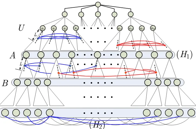
The graph we construct will contain a smaller explicit expander on a fixed proportion of its vertices, connected to what is essentially a product of another expander with a “stretched” regular tree (one where the edges in certain levels are replaced by paths).
Leth→ ∞and letH1,H2be two explicit expanders as follows (cf. e.g.[1]for an explicit construction
of a 3-regular graph, as well as[18]and the references therein for additional explicit constructions of constant-degree expander graphs):
• H1: An explicit 3-regular expander on 20·22hvertices.
• H2: An explicit 4-regular expander on 20·26hvertices.
Letλ(Hi) denote the largest absolute-value of any nontrivial eigenvalue ofHi fori=1, 2. Finally, let Lbe some sufficiently large fixed integer whose value will be specified later.
Our final construction for 5-regular expander will be based on a (modified) regular tree, hence it will be convenient to describe its structure according to the various levels of its vertices. Let the vertexρdenote the root of the tree, and construct the graphG as follows:
1. Levels 0, 1, 2: First levels of a 5-regular tree rooted atρ.
• Denote byU={u1, . . . ,u20}the vertices comprising level 2.
2. Levels 3, . . . ,h+2: Stretched 4-ary trees rooted at each vertex ofU, defined as follows:
• For eachui ∈U place anh-level 4-ary treeTui rooted at ui and identify the vertices of Tui andTuj via the trivial isomorphism.
• Replace every edge of eachTui by a (disjoint) path of lengthL.
Connect Tu∗1, the new interior vertices in Tu1 (with initial degree 2) to their isomorphic
counterparts inTu∗2,T ∗ u3,T
∗
u4(add 4-cliques between identified interior vertices) and similarly
u1 u2 u3
. . . . .
u17 u18 u19 u20U
A
. . .
(
H
1
)
u4
. . .
B
(
H
2)
L
L
. . . . .
. . . . .
. . . . .
. . .
. . .
. . .
Figure 1: Explicit construction of a 5-regular graph on which the random walk exhibits total-variation cutoff.
• LetAdenote the final 20·4h vertices comprising levelh+2, and associate the vertices ofA
with those ofH1.
3. Levelsh+3, . . . , 2h+2: Product ofH1 and a stretched 4-ary tree, defined as follows:
• For eacha∈Aplace anh-levelL-stretched 4-ary treeTa.
Connect vertices inTa∗with their counterparts inTb∗fora b∈E(H1).
• LetB denote the final 20·42hvertices comprising level 2h+2.
4. Levels 2h+3, . . . , 3h+2: A forest of 4-ary trees rooted at each vertex ofB.
5. Last level: Associate leaves withH2 and interconnect them accordingly.
Finally, the aforementioned parameterLis chosen as follows: Denote by
gap1= inf
|H1|
1−λ(H1)/3
, gap2=inf
|H2|
1−λ(H2)/4
the minimum spectral-gaps in the explicit expanders that were embedded in our construction (re-calling from the introduction thatgapi>0 for both i=1, 2 by the definition of expanders together with the discrete analogue of Cheeger’s inequality), and define
L=
2
pgap 1
∨ 16
gap2 ∨ 32
. (2.1)
See Fig. 1 for an illustration of the above construction.
For some insight to the various building blocks of the construction, observe that the height of the
SRW on a regular tree behaves as a one-dimensional biased random walk with the bias in the
SRWmixes once it is reaches the leaves and is approximately uniform on its level. When the walk
is started from the firsth+2 levels, the addition of the expander H1 ensures that it is uniform on
its level by the time it reaches the leaves. Walks started from below levelh+2 are not necessarily mixed upon reaching the leaves yet subsequently mix after that point due to the expanderH2 in a total time which is strictly less than the time it takes the walk from the root to merely reach the leaves. Our construction thus ensures that the root is the worst case starting position for mixing and that theSRWstarted at it exhibits cutoff.
We begin by establishing the expansion of the above constructedG. Throughout the proof we omit ceilings and floors in order to simplify the exposition.
Lemma 2.1. Letκ= (ch(H2)∧1)/3for H2 our explicit4-regular expander. For any integer L>0, the Cheeger constant of the above described5-regular graph G with parameter L satisfiesch(G)≥κ/25L. Moreover, the induced subgraphG on the last h levels (i.e., levels˜ 2h+2, . . . , 3h+2) hasch(G˜)≥κ. Proof. First consider the entire graphG. Since we are only interested in a lower bound on ch(G), clearly it is valid to omit edges from the graph, in particular we may erase the cross edges between any subtreesTu∗,Tv∗described in Items 2,3 of the construction. This converts every stretched edge of the 5-regular tree of G simply into a 2-path (one where all interior vertices have degree 2) of length L.
Next, we contract all the above mentioned 2-paths into single edges and denote the resulting graph byF. The next simple claim shows that this decreases the Cheeger constant by at mostO(L).
Claim 2.2. Let F be a connected graph with maximal degree∆ and let G be a graph on at most 32|F| vertices obtained via replacing some of the edges of F by2-paths of length L. Thench(G)≥ch(F)/∆2L. Proof. LetX ⊂V(G)be a set of cardinality at most|G|/2 achieving the Cheeger constant of G. We may assume that ∆ ≥ 3 otherwise F is a disjoint union of paths and cycles and the result holds trivially.
Notice that ifX contains two endpoints of a 2-pathP = (x0, . . . ,xL)while only containingk<L−1 interior vertices ofP then we can assume thatX∩ P ={x0, . . . ,xk,xL}, i.e. all the interior vertices are adjacent (this maintains the same cardinality ofX while not increasing∂X). With this in mind, modify the setX into the setX′by repeating the following operation: As long as there is a 2-pathP
as above (withx0, . . . ,xkandxLinX for somek<L−1) we replacexLby xk+1. This maintains the cardinality of the set while increasing its edge-boundary by at most∆−2 (asxLformerly contributed
at least 1 edge to this boundary due to xL−1∈/ X). Altogether, this yields a setX′where no 2-path P = (x0, . . . ,xL)*X′has bothx0,xL∈X′, whileX′satisfies
|∂X′|/|X′| ≤(∆−1)ch(G).
The obtained subsetX′is possibly disconnected, and we will next argue that its connected compo-nents satisfy an appropriate isoperimetric inequality. ConsiderX′′, the connected component of X′
that minimizes|∂X′′|/|X′′|. If X′′is completely contained in the interior of one of the new 2-paths then the statement of the claim immediately holds since
ch(G)≥ |∂X
′|
(∆−1)|X′| ≥
|∂X′′|
(∆−1)|X′′| ≥
2
(L−1)(∆−1) ≥
with the last inequality due to the fact ch(F)≤∆. Suppose therefore that this is not the case hence we may now assume thatX′′contains at least one endpoint of any 2-path it intersects.
LetY =X′′∩V(F), i.e. the subset of the vertices ofF obtained fromX′′by excluding any vertex that was created inGdue to subdivision of edges. Observe that our assumption onX′implies that
|∂Y|=|∂X′′|,
since either a 2-path P is completely contained in X′′ (not contributing to ∂X′′) or P ∩X =
{x0, . . . ,xk} for some k < L (contributing the edge xk,xk+1 to ∂X′′, corresponding to the edge x0,xL in∂Y).
It remains to consider|Y|. Clearly, X′′ can be obtained from Y by adding at most ∆new 2-paths withL−1 new interior points per vertex, hence
|Y| ≥ |X′′|/∆L.
On the other hand, since|Y| ≤ |X′′| ≤ |G|/2 and|G| ≤ 32|F|we have
|Y|/|F| ≤ 32|X′′|/|G| ≤ 34, which together with the fact that|X′′| ≤ |G|/2 implies that
|V(F)\Y| ≥1 4|F| ≥
1 6|G| ≥
1 3|X
′′| ≥ |X′′|/∆L.
Altogether,
ch(F)≤ |∂Y|
|Y| ∧ |V(F)\Y| ≤∆L |∂X′′|
|X′′| ≤∆
2Lch(G).
In light of the above claim we have ch(G)≥ch(F)/25L where the graphF is the result of taking a complete 5-regular tree of height 3h+2 levels and connecting its 5·43h+1leaves, denoted byF′, via the 4-regular expanderH2. It therefore remains to show that ch(F)≥κ.
LetSbe a set of sizes≤ |F|/2 vertices that achieves ch(F). Define its subset of the leavesS′=S∩F′
and sets′=|S′|. Since|F′| ≥ 34|F| we clearly haves′≤s≤ 23|F′|hence |S′| ∧ |F′\S′|
≥s′/2. We thus have the following two options:
1. s′≥ 23s: In this case
|∂FS| ≥ |∂F′S′| ≥ch(H2)s′/2≥ch(H2)s/3 .
2. s′< 23s: LettingT5 denote the infinite 5-regular tree (whose Cheeger constant equals 3) we get
|∂FS| ≥ch(T5)(s−s′)−s′=3s−4s′>s/3 . Altogether we deduce that
ch(G)≥ch(F)≥(ch(H2)∧1)/3=κ.
Consider theSRWstartedk≤hlevels above the bottom (i.e. at level 3h+2−k) of the graphG. The
height of the walk is then a one-dimensional biased random walk with positive speed 3
5, implying
that it would reach the bottom after 53k+o(h)steps with high probability.
On the other hand, if theSRW is started closer to the root, i.e. at level 2h+2−k, then the
one-dimensional random walk is delayed by two factors, horizontal (cross-edges) and vertical (stretching the edges into paths). Until reaching level 2h+2 (after which the previous analysis applies), these delays are encountered along 53k+o(h)stretched edges with the following effect:
• The former incurs a laziness delay with probability 35 whenever the walk is positioned on an interior vertex of a 2-path.
• The latter delays the walk by the passage time of aSRWthrough anL-long 2-path, where the
walk leaves the origin with probability 1.
It is well-known (and easy to derive) that the expected passage time of the one-dimensionalSRW
from 0 to±Lis precisely L2 and the expected number of visits to the origin by then (including the starting position) is exactly L. It thus follows that the expected delay of the one-dimensional walk representing our height in the tree along a single stretched edge is
5 2(L
2
−L) +L= 12L(5L−3).
Combining the above cases we arrive at the following conclusion:
Claim 2.3. Consider the SRW on the graph G started at a vertex on level s ∈ {0, . . . , 3h+1}. Set
α=s/h and letτℓbe the hitting time of the walk to the leaves (i.e. to level3h+2). Then w.h.p.
τℓ=
¨
(5
3+o(1))
L(5L−3)(1−α2) +1h If0≤α≤2 ,
5
3(3−α)h+o(h) Ifα≥2 .
The next lemma relatesτℓ, the hitting time to the leaves (addressed by the above claim), and the mixing of theSRWon the graph.
Lemma 2.4. Letǫ >0, let s0 be some vertex on level l0 ∈ {0, . . . ,h+2}and T = (1+δ)Es 0τℓ for
δ >0fixed, whereτℓ is the hitting time of theSRW to the leaves. ThenkPs0(ST ∈ ·)−πkTV < ǫfor any sufficiently large h.
Proof. Let(St) denote theSRW started at some vertexs0 in level l0 ≤h+2 andπbe the uniform
distribution onV(G). Let(S˜t)be a random walk started from the uniform distribution ˜S0∼π. Write Lifori∈ {0, . . . , 3h+2}for the vertices of leveliinG(accounting for all the vertices except interior
ones along the 2-paths of lengthLcorresponding to stretched edges) and letψ:G→ {0, . . . , 3h+2} map vertices in the graph to their level (while mapping interior vertices of 2-paths to the lower of their endpoint levels).
Further letΩ ={2h+3, . . . , 3h+2}. Clearly, for large enoughhwe have
P ψ(S˜0)∈/Ω < ǫ
10.
Furthermore, due to the bias of theSRWtowards the leaves and the fact thatτℓ= (1+o(1))Eτℓ≍h
(recall Claim 2.3 and thatL is fixed) we deduce thatψ(ST)> 52hexcept with probability exponen-tially small inh, and in particular for any sufficiently largeh
P ψ(ST)∈/Ω < ǫ
Therefore, an elementary calculation shows that ifψ(ST)andψ(S˜T)are close in total-variation and
a product of a 4-ary tree whose edges are stretched into L-long 2-paths and the expanderH1. Let
ϕ:G→H1 map the vertices in these levels to their corresponding vertices inH1, and letτ0,τ1 be
the hitting times of(St)to levels 32hand 2h+2 respectively.
As argued above, theSRWstarted at level 2h+2−kis a one-dimensional biased random walk that
w.h.p. passes through(1+o(1))5
whenever it is in an interior vertex in the 2-path, for a total expected number of 3
2(L 2
−L) such moves.
Finally, due to its bias towards the leaves, with high probability theSRWfrom level3
2hreaches level
2h+2 (the vertices B) before hitting levelh+2. Applying CLT we conclude that theSRWw.h.p.
traverses
(54+o(1))L(L−1)h>L2h
cross-edges (each corresponding to a single step of theSRW on H1) between timesτ0,τ1, where
the last inequality holds for L > 5 and large enough h. This amounts to at least L2hconsecutive steps of aSRWalongH1.
Aiming for a bound on the total-variation mixing, we may clearly condition on events that occur with high probability: Condition therefore throughout the proof that indeed the above statement holds.
Recalling thatH1is a 3-regular with second largest (in absolute value) eigenvalueλ(H1)and writing
with the last inequality justified for any sufficiently largehprovided that
L> p
5 log 2
p
1−λ(H1)/3
, (2.4)
a fact inferred from the choice ofLin (2.1). In this case, for anys0
Ps 0
Sτ1=u
=1+o(1)
|A| for everyu∈A.
By symmetry we now conclude that for anyi∈Ωandt≥τ1 we have Ps
0 St∈ · |ψ(St) =i
= 1+o(1)
|Li|
for everyi∈ {2h+2, . . . , 3h+2} .
This immediately establishes (2.2).
To obtain (2.3), note that ˜St for t = τ1 w.h.p. satisfies ψ(S˜0) > 52h. Conditioned on this event
we can apply a monotone-coupling to successfully couple(St)and(S˜t)such thatψ(Sτℓ) =ψ(S˜τℓ), yielding (2.3).
The concentration of τℓ established in Claim 2.3 carries the above two bounds to time T, thus
completing the proof.
LettMIX(ǫ;x)denote the total-variation mixing time from a given starting position x. That is, if(Xt)
is an ergodic Markov chain on a finite state spaceΩwith stationary distributionπthen
tMIX(ǫ;x) △
=min
t:kPx(Xt∈ ·)−πkTV< ǫ .
The above lemma gives an upper bound on this quantity for theSRW started at one of the levels {0, . . . ,h+2}, which we now claim is asymptotically tight:
Corollary 2.5. Consider the SRW on G started at some vertex s0 on level l0 ∈ {0, . . . ,h+2}and let
τℓ be the hitting time of the walk to the leaves. Then for any fixed0< ǫ < 1we have tMIX(ǫ;s0) =
(1+o(1))Es 0τℓ.
Proof. The upper bound ontMIX(ǫ;s0)was established in Lemma 2.4.
For a matching lower bound on tMIX(1−ǫ;s0)choose some fixed integer K=O(log(L/ǫ))such that
the bottomK levels of the graph comprise at least a(1−ǫ)-fraction of the vertices ofG, i.e.
X
i>3h+2−K
Li
>(1−ǫ)|G|.
The lower bound now follows from observing that, by the same arguments that established Claim 2.3, the hitting time from level l0 to level 3h+2−K is w.h.p. (1−o(1))Eτℓ for any
suf-ficiently largeh.
Having established the asymptotic mixing time of theSRWstarted at the tophlevels, we next wish
Claim 2.6. Let(St)be theSRW started at some vertex x in levelψ(x)>h. For every0< ǫ <1and any sufficiently large h we have tMIX(ǫ;x)<6L
2h.
Proof. Let G′ denote the induced subgraph on the bottom h+1 levels of the graph (i.e., levels 2h+2, . . . , 3h+2). Since |G′| = (1−o(1))|G| it clearly suffices to show that (St) mixes within total-variation distanceǫonG′.
By Claim 2.3 (taking the worst caseα = 1 corresponding toψ(x) =h) with high probability we have
τℓ≤(56+o(1))[L(5L−3) +2]h<5L2h
△
=t1,
where the above strict inequality holds for any sufficiently largeh(as L≥1).
Recall that ch(G′)≥κ= (ch(H2)∧1)/3 by Lemma 2.1, whereH2 is the explicit 4-regular expander
with second largest (in absolute value) eigenvalueλ(H2). Further consider the graph G′′obtained
by adding toG′a perfect matching on level 2h+2, thus making it 5-regular. Clearly, adding edges can only increase the Cheeger constant and so ch(G′′) ≥ κ as well. Moreover, the discrete form of Cheeger’s inequality ([5, 6, 12, 20]), which for a d-regular expander H with second largest (in absolute value) eigenvalueλstates that
d−λ
(the strict inequality holding for large enoughh) steps we have
max
time, and thereafter (due to its bias towards the leaves) it does not revisit level 2h+2 until time
t1+t2 except with a probability that is exponentially small in h. Since G and G′′ are identical
in G′′ following τℓ. Altogether, for large enough hwe have
Px
St1+t2∈ ·
−π
TV < ǫ and so tMIX(ǫ;x)<t1+t2.
Finally, bearing (2.5) and the choice of Lin (2.1) in mind,
L≥ 64
4−(λ(H2) ∨ 2)>
Æ9
4·6 p
50
4−(λ(H2) ∨ 2), (2.6)
hence L2>9/4γand sot2≤L2handt1+t2≤6L2h, as required.
We now claim that the worst-case mixing time within any 0< ǫ <1 is attained by an initial vertex at distanceo(h)from the root. Fix 0< ǫ <1, letx be the initial vertex maximizingtMIX(ǫ;x)and recall
thatψ(x) denotes its level in the graph. The combination of Claim 2.3 and Corollary 2.5 ensures that ifψ(x)≤hthen necessarilyψ(x) =o(h), in which case
tMIX(ǫ;x) =
5
3+o(1)
(5L2−3L+1)h=△ t⋆. (2.7)
An immediate consequence of the requirement 2.6 on L is that L ≥ 50, hence t⋆ > 8L2hfor any sufficiently largeh. Therefore, we cannot haveψ(x)>hsince by Claim 2.6 that would imply that
tMIX(ǫ;x)<6L
2hcontradicting the fact thatx achieves the worst-case mixing time.
Overall we deduce that for any 0< ǫ <1 we have
tMIX(ǫ) =max
x tMIX(ǫ;x) = (1+o(1))t
⋆,
thus confirming that theSRWon the above constructed family of 5-regular expanders exhibits
total-variation cutoff from a worst starting location.
It remains to describe how our construction can be (relatively easily) modified to be 3-regular rather than 5-regular.
The immediate step is to use binary trees instead of 4-ary trees, after which we are left with the problem of embedding the explicit expandersH1andH2without increasing the degree. This will be achieved via the line-graphs of these expanders, hence our explicit expanders will now have slightly different parameters:
• H1: An explicit 3-regular expander on 2h+1 vertices.
• H2: An explicit 3-regular expander on 23h+1vertices.
Recall that given a tree rooted at some vertexu, denoted byTu, its edge-stretched version is obtained
by replacing each edge by a 2-path of length L, and the collection of all new interior vertices (due to subdivision of edges) is denoted byTu∗. The modified construction is as follows:
1. Levels 0,1,2: First levels of a binary tree.
• Denote byU ={u1, . . . ,u6}the vertices in level 2.
• Connect vertices fromTu∗
i (interior vertices along 2-paths) to the corresponding (isomor-phic) vertices inTu∗
2i, i.e. inter-connect the interior vertices via perfect matchings. • Denote byAthe 6·2hvertices in levelh+2.
3. Levelsh+3, . . . , 2h+2: Edge-stretched binary trees rooted at Aand inter-connected via the line-graph ofH1 using auxiliary vertices:
• Associate each binary treeTa
i rooted atAto anedgeofH1.
• For each x ∈ Ta∗i (interior vertex on a 2-path) we connect it to a new auxiliary vertex x
′
and associate x′with a unique edge ofH1.
• We say that x ∈ Ta∗
i and y ∈ T
∗
aj are isomorphic if the isomorphism from Tai to Taj mapsx to y. Add|H1|new auxiliary vertices per equivalence class of|A|such isomorphic
vertices, identify them with the vertices of H1 and connect every new vertex v to the auxiliary vertices x′,y′,z′representing the edges incident to it.
4. Levels 2h+3, . . . , 3h+2: A forest of binary trees.
5. Last level: leaves are inter-connected via the line-graph ofH2:
• Associate the 6·23hvertices with the edges ofH2.
• Add|H2|new auxiliary vertices, each connected to the leaves corresponding to edges that are incident to it inH2.
It is easy to verify that the walk along the cross-edges of theTa∗i’s now corresponds to a lazy (un-biased) random walk on the edges of H1. Similarly, the walk along the cross-edges connecting the leaves corresponds to the SRW on the edges of H2. Hence, all of the original arguments
re-main valid in this modified setting for an appropriately chosen fixedL. This completes the proof of
Theorem 1.
2.2
Explicit expanders without total-variation cutoff
The explicit cubic expanders with cutoff constructed in the previous section (illustrated in Fig. 1) can be easily modified so that theSRWon them from a worst starting position would notexhibit
total-variation cutoff.
To do so, recall that in the above-described family of graphs, each vertex of the subsetU was the root of a regular tree of height hwhose edges were stretched into L-long 2-paths (see Item 2 of the construction). We now tweak this construction by stretching some of the edges into 2-paths of length L′. Namely, for subtrees rooted at theodd vertices in levelh/2 of these trees we stretch the edges into paths of length L′> L. Under this modified stretching the trees Tu
i are clearly still isomorphic, hence the cross edges are inter-connecting 2-paths of the same lengths.
G
. . .
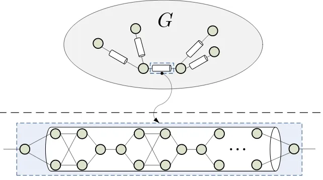
Figure 2: Extension of the explicit expanders with cutoff to graphs with prescribed order of cutoff location.
distinct values (differing by a fixed multiplicative constant), each with probability 12 −o(1). This implies that the ratio tMIX(
1 4)/tMIX(
3
4)is bounded away from 1 and in particular this explicit family
of expanders does not have total-variation cutoff.
2.3
Proof of Theorem 2: cutoff at any prescribed location order
Suppose H is an explicit 3-regular expander on mvertices provided by Theorem 1, and recall that theSRWon this graph exhibits cutoff atClogmwhereC >0 is some absolute constant. Our graph G will be the result of replacing every edge of H by the 3-regular analogue of a 2-path, which we refer to as a “cylinder”, illustrated in Fig. 2. The length of each cylinder is set to be L = L(m)
satisfyingL≡1 (mod 4). Notice that the total number of vertices inG is
n=|V(H)|+|E(H)|3
2(L−1) =
1+9
4(L−1)
m. (2.8)
Sincem→ ∞and theSRWonH, started at a worst-case starting position, traverses(C+o(1))logm
edges until mixing, we infer from CLT, as well as the fact that the expected passage-time through an
L-long cylinder isL2, that the analogous random walk onG has cutoff at
tMIX=C L
2logm= (C+o(1))L2log(n/L). (2.9)
When L(m) = O(1) we have tMIX ≍ logn. On the other extreme end, when L grows arbitrarily
fast as a function of mwe obtain that it approaches n arbitrarily closely but we must still having
L = o(n) since n/L ≍ m → ∞. In that case tMIX approaches n
2 arbitrarily closely while having a
strictly smaller order.
To complete the construction it remains to observe that we may choose L andm so that|Gn| ≍n
andtMIX ≍tn. This can be achieved by first selecting Lso thattn≍(C+o(1))L2log(n/L)and then
To show that there is no cutoff whenever tMIX ≍n
2 we will argue that in that case we havegap= O(n−2), in contrast to the necessary condition for cutoff gap−1 = o(tMIX) due to Peres (cf. [16]),
discussed in the introduction.
Lemma 2.7. Let G be a graph on n vertices with degrees bounded by some∆fixed on which theSRW has tMIX≍n
2. Then the spectral-gap of the walk satisfiesgap
≍n−2. In particular, theSRWon G does not exhibit cutoff.
Proof. Observe that the above graph must satisfy diam(G)≥ cnfor some fixed c >0 as it is well-known (cf., e.g.,[4]) that the lazy walk on any graph H has tMIX =O(diam(H)vol(H)) and in our
case vol(G)≤∆n=O(n).
Let x,y∈V(G)be two vertices whose distance inG is
N=△ distG(x,y) =diam(G)≥cn.
Our lower bound on the gap will be derived from its representation via the Dirichlet form, according to which
gap=inf
f
E(f)
Var(f) =inff 1 2
P
x,y∈Ω
f(x)− f(y)2
π(x)P(x,y)
Varπf
, (2.10)
whereπ is the (uniform) stationary measure andP is the transition kernel of theSRW. As a
test-function f :V(G)→Rin the above form choose
f(v)=△distG(x,v).
Clearly we haveE(f)≤1 and a lower bound of ordern2on the variance follows from the fact that two sets of linear size each have a linear discrepancy according to f. Namely,
πf−1({0, . . . ,⌊N/4⌋})≥ c
4 , π
f−1({⌈3N/4⌉, . . . ,N})≥ c
4,
as a result of which
Var(f)≥(c/4)(N/4)2>c′n2.
We conclude thatgap=O(n−2), thus completing the proofs of Lemma 2.7 and Theorem 2.
3
Concluding remarks and open problems
• Recent results in [15] showed that almost every regular expander graph has total-variation cutoff (prior to that there were no known examples for bounded-degree graphs with this phe-nomenon); here we provided a first explicit construction for bounded-degree expanders with cutoff.
• A slight variant of our construction gives an example of a family of expanders where theSRW
does not exhibit cutoff, thereby disagreeing with Peres’ cutoff-criterion. Both here and in an-other such example due to Peres and Wilson[17]the expanders are non-transitive (hence the restriction to transitive graphs in Peres’ conjecture stated next).
• While it is conjectured by Peres that the random walk on any family of transitive bounded-degree expanders exhibits total-variation cutoff, there is not even a single example of such a transitive family where cutoff was proved (or disproved).
• For general (not necessarily expanding) bounded-degree graphs on nvertices it is well-known that tMIX =O(n
2). Here we showed that cutoff can occur essentially anywhere up to o(n2)by
constructing cubic graphs with cutoff at any such prescribed location. Furthermore, this is tight as we prove that if tMIX≍n
2 then cutoff cannot occur.
Acknowledgment
We would like to thank Yuval Peres for suggesting the problem, his encouragement and useful discussions.
References
[1] M. Ajtai,Recursive construction for3-regular expanders, Combinatorica14(1994), no. 4, 379–416.
[2] D. Aldous,Random walks on finite groups and rapidly mixing Markov chains, Seminar on probability, XVII, 1983, pp. 243–297.
[3] D. Aldous and P. Diaconis,Shuffling cards and stopping times, Amer. Math. Monthly93( 1986 ), 333–348.
[4] D. Aldous and J. A. Fill,Reversible Markov Chains and Random Walks on Graphs. In preparation,http://www.stat. berkeley.edu/~aldous/RWG/book.html.
[5] N. Alon,Eigenvalues and expanders, Combinatorica6(1986), no. 2, 83–96.MR875835
[6] N. Alon and V. D. Milman,λ1,isoperimetric inequalities for graphs, and superconcentrators, J. Combin. Theory Ser. B
38(1985), no. 1, 73–88.MR782626
[7] N. Berestycki,Phase transitions for the distance of random walks and applications to genome rearrangement, Ph.D. dissertation, Cornell University (2005).
[8] G.-Y. Chen and L. Saloff-Coste,The cutoff phenomenon for ergodic Markov processes, Electronic Journal of Probability 13(2008), 26–78.
[9] P. Diaconis,The cutoff phenomenon in finite Markov chains, Proc. Nat. Acad. Sci. U.S.A.93(1996), no. 4, 1659–1664.
[10] P. Diaconis and M. Shahshahani,Generating a random permutation with random transpositions, Z. Wahrsch. Verw. Gebiete57(1981), no. 2, 159–179.
[11] J. Ding, E. Lubetzky, and Y. Peres,Total-variation cutoff in birth-and-death chains, Probab. Theory Related Fields146 (2010), no. 1, 61–85.
[12] J. Dodziuk,Difference equations, isoperimetric inequality and transience of certain random walks, Trans. Amer. Math. Soc.284(1984), no. 2, 787–794.MR743744
[13] R. Durrett,Random graph dynamics, Cambridge Series in Statistical and Probabilistic Mathematics, Cambridge Uni-versity Press, Cambridge, 2007.
[14] S. Hoory, N. Linial, and A. Wigderson,Expander graphs and their applications, Bull. Amer. Math. Soc.43(2006), no. 4, 439–561.MR2279667
[16] Y. Peres, American Institute of Mathematics (AIM) research workshop “Sharp Thresholds for Mixing Times” (Palo Alto, December 2004).
[17] Y. Peres and D. B. Wilson. Private communication.
[18] O. Reingold, S. Vadhan, and A. Wigderson,Entropy waves, the zig-zag graph product, and new constant-degree ex-panders, Ann. of Math. (2)155(2002), no. 1, 157–187.
[19] L. Saloff-Coste,Random walks on finite groups, Probability on discrete structures, 2004, pp. 263–346.