PERFORMANCE OF LOGISTIC REGRESSION MODEL
AND SPATIAL METHOD
(Case: Predicting of Deforestation in
Cikepuh Wildlife Reserve
and Cibanteng Natural Reserve)
d
GRADUATE SCHOOL
PERFORMANCE OF LOGISTIC REGRESSION MODEL
AND SPATIAL METHOD
(Case: Predicting of Deforestation in
Cikepuh Wildlife Reserve
and Cibanteng Natural Reserve)
BONIE FAJAR DEWANTARA
A thesis submitted for the degree of Master of Science of Bogor Agricultural University
GRADUATE SCHOOL
STATEMENT
I am Bonie Fajar Dewantara stated that this thesis entitled :
Performance of Logistic Regression Model and Spatial Method (Case: Predicting of Deforestation in Cikepuh Wildlife Reserve and
Cibanteng Natural Reserve)
is result of my own works during the period January 2005 – September 2006 and
it has not been published before. The contents of thesis have been examined by
the advising committee and an external examiner.
Bogor, September 2006
ACKNOWLEDGEMENT
Alhamdulillah, Thanks to God, at the last this thesis has finished
successfully, and I would like to thank to all people who have helped and assisted
me during finishing the thesis. There are many people I should thank in regard to
this work and no doubt I will not be able to mention them one by one, and I can
buy beg forgiveness.
I deeply appreciate the efforts and thank to my supervisor Dr. Ir. Lilik
B. Prasetyo, M.Sc and co-supervisor Idung Risdiyanto S.Si, M.Sc for their
guidance, technical, comments and constructive criticism through all months of
my research. My special gratitude also goes to Dr. Ir. I Nengah Surati Jaya, M.Sc
as the external examiner and Dr. Ir. Hatrisari Hardjomidjojo, DEA, as the seminar
and examination chairman (moderator) for their positive ideas, inputs, and
criticism. And also my special gratitude goes to all my teachers, my lectures for
sharing their knowledge and experiences.
I would like to thank to SEAMEO-BIOTROP management and staff,
especially Dr. Ir. Tania June, M.Sc and MIT staff and management, technical and
facility. Especially To Devi, Uma, and Bambang; Pak Jejen has been together
gone to the field to collect ground truth data, and also Pak Asep in Ciracap for his
home stay. Also, I thank to PPLH (Pusat Penelitian Lingkungan Hidup /
Environmental Research Center) Bogor Agricultural University for the image data
and Baplan (Badan Planologi / Forestry Planning Agency) Ministry of Forestry,
for digital map data I would like to thank to Conservation International –
Indonesia for the basic idea of image processing methodology and Wildlife
Conservation Society – Indonesia Program for the ERDAS Imagine 8.7 and
ArcView license usage. For my friends in MIT especially in the same batch
2002, I really appreciate our togetherness, our 24-hours-a-day works, and how to
Finally I feel deeply indebted to my lovely dear wife, Frida Yuliyanti
S.Hut for her moral support and patience during the course, and especially also for
both my sons Ariodanie Fudhail Hanif and Ariq Maulana Malik Ibrahim; my
parents Adnan Hanif (alm) and Hj. Chadidjah, and all my family. I dedicated this
thesis for the glory of knowledge and science of Indonesia.
Bonie Adnan
CURRICULUM VITAE
Bonie Fajar Dewantara was born in Belawan –
Medan, North Sumatera, Indonesia at January 1st, 1971. He
received his undergraduate diploma from Bogor Agricultural
University in 1996, especially Forest Product Technology
Department of Forestry Faculty.
Since 1996 to 1999 he worked at Risjad Salim International Bank, and
from 1999 to 2002 worked at Carrefour Indonesia as Department Head, and from
2002 to 2004 worked at Ritel and Logistic Consultant PT. Wira Prima Abadi, and
continued to consultant firm PT. Explorer Indonesia from 2004 – 2005 as Head of
Forestry Division. Now, he has been working at Wildlife Conservation Society –
Indonesia Program as GIS and Remote Sensing Analyst since 2005.
In 2002, he registered as a post-graduated student of Bogor Agricultural
University, program study Master of Science in Information Technology for
Natural Resources Management, and received his post-graduated diploma in 2006
with thesis title “Performance of Logistic Regression Model and Spatial Method
(Case: Predicting of Deforestation in Cikepuh Wildlife Reserve and Cibanteng
ABSTRACT
BONIE FAJAR DEWANTARA (2006). Performance of Logistic Regression Model for Predicting Deforestation, Case Study: Cikepuh Wildlife Reserve and Cibanteng Natural Reserve. Under the supervision of LILIK BUDI PRASETYO and IDUNG RISDIYANTO.
Cikepuh Wildlife Reserve and Cibanteng Natural Reserve, since both conservation area was established in 1973 and 1925 have been facing complex problem caused by land use changed, deforestation, illegal hunting, forest fire, and so on. Deforestation itself is a complex socio-economic, cultural, and political event. This thesis focused on what factors affect the rate of deforestation by considering some common driving forces of deforestation and using logistic regression for predicting deforestation. It is clearly important to know where deforestation is likely to occur. The objectives of the thesis are to quantify the contribution of each deforestation driving factor such as distance from center of dweller, aspect, slope, distance from shore line, distance from existing road, and elevation, and to elaborate spatial projection of future trends of deforestation based on possibility of deforestation as the result of logistic regression equation.
The methodology is using Stacking Method from CI (Conservation International) CABS (Center for Biodiversity Applied Science) and developed together with WCS IP (Wildlife Conservation Society – Indonesia Program). Two image with different dates or one period was stacked and analyzed by visualization from both images. Signature area was extracted from the stacked-images by using shapefile polygon for forest to forest class, forest to non forest class, non to non forest class, water, cloud and shadow. Signature area should be represented certain spectral characteristic, so for obtaining number of class as many as possible, it could use 16 bit data type indeed 8 bits.
Classification method is supervised classification that was done by CART ERDAS Imagine plug in tool and See5, a stand alone decision-tree based classification program. The result of classification is thematic raster image with forest change attribute. Analysis was done in one attribute table of polygon vector cell (PVC), that is created by using Edit Tool Vector Grid, an extension from ArcView 3.3. All attribute of independent variables fill the squared-shaped polygon as called PVC, and the result probability of logistic regression as the result of the calculation as well.
Independent variable is divided to two binary category 0 and 1. 1 is a parameter that tends to occur deforestation such as less 1 km distance from road. 0 is stable condition that there is no change from forest to non forest. The result of possibility deforestation occurrence is if the road distance less than 1 km, tends to deforested occurrence 3 times compare the distance greater or equal 1 km. The smallest possibility of deforestation occurrence was contributed by predictor distance 1 km from river, and almost has no effect to deforested occurrence.
Research Title : Performance of Logistic Regression Model and Spatial Method (Case: Predicting of Deforestation in Cikepuh Wildlife Reserve and Cibanteng Natural Reserve)
Name : Bonie Fajar Dewantara
Student ID : G.051020051
Study Program : Master of Science in Information Technology for
Natural Resources Management
Approved by,
Advisory Board
Dr. Ir. Lilik Budi Prasetyo, M.Sc Idung Risdiyanto, S.Si, M.Sc Supervisor Co-supervisor
Endorsed by,
Program Coordinator Dean of Graduate School
Dr. Ir. Tania June, M.Sc Prof. Dr. Ir. Khairil A. Notodiputro, MS
TABLE OF CONTENTS
Page
Table of Content ……… ……… i
List of Figure ……….. iii
List of Table ………..………. vi
List of Appendix ………..……….. vii
I INTRODUCTION 1.1. Background ……… 1
1.2. Obejctives ……… 2
1.3. Hypothesis ………. 3
II LITERATURE REVIEW 2.1. Logistic Regression Model ……… 4
2.1.1. Logistic Regression Equation ……… 6
2.1.2. Significance Test for Parameter Predictors ……… 7
2.1.3. Model Interpretation ……… 9
2.1.4. Logistic Regression Coefficient and Correlation ………… 11
2.2. Remote Sensing, GIS and Change Detection ……… 12
2.2.1. Remote Sensing ……… 12
2.2.2. Change Detection……… 12
2.3.3. Geographical Information System ……… 13
2.3. Deforestation ……… 14
III MATERIALS AND METHODS 3.1. Time and Location ………... 16
3.2. Data Sources ……… 17
3.3. Supporting Tools / Program ………. 18
3.4. Methodology………. 19
3.4.1. Image Preprocessing………... 19
b. Geo-Referencing ……… 19
3.4.2. Image Processing ……… 21
a. Image Stacking……….. 21
b. Signature Area ……… 22
c. ERDAS Imagine – CART Classification ………….…… 24
3.4.3. Vector Processing ……….. 26
a. Creating Cell Vector……….. 26
b. Extracting Variables Data ………. 27
3.4.4. Logistic Regression Model ……… 29
3.5. Assumption of Research Study ……….. 30
IV RESULTS AND DISCUSSION 32 4.1. Image Processing ……… 32
4.1.1. Period 1990 - 1997………. 32
4.1.2. Period 1997 - 2001 ……… 37
4.2. Vector Processing ………. 40
4.2.1. Creating Vector Cell ……… 40
4.2.2. Data Extracting of Contour SRTM Data Image ... 41
4.2.3. Data Extracting of River Buffer Process ……… 43
4.2.4. Data Extracting of Road Buffer Process ………... 44
4.2.5. Data Extracting of Shoreline Buffer Area Process ………. 45
4.2.6. Data Extracting of Pupolation Center Buffer Area Process . 46 4.2.7. Data Extracting of Aspect Area Image ……… 48
4.2.8. Data Extracting of Slope Area Image ………. 50
4.3. Logistic Regression ……… 51
4.3.1. Logistic Regression Equation ……… 51
4.3.2. Significance Test of Model and Predictors ………. 53
4.3.3 Logistic Coefficient and Correlation ……… 59
4.4. Validation and Accuracy Assessment ………... 61
4.4.1. Validation ……… 61
V CONCLUSION AND RECOMMENDATION 66
5.1. Conclusion ……… 66
5.2. Recommendation ……… 67
REFERENCES 69
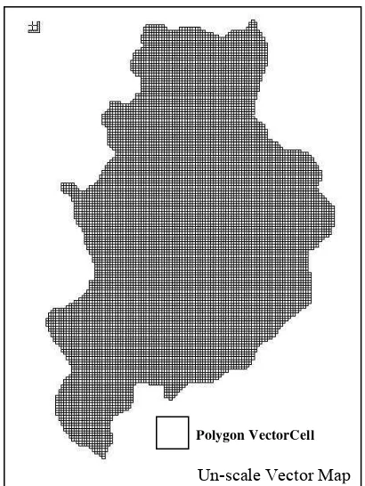
Appendix 1. Vector Map of Study Area ………... 74
Appendix 2. Illustration of attribute table in spatial processing ……... 75
Appendix 3. SPSS Output ………. 76
LIST OF FIGURE
No Caption Page
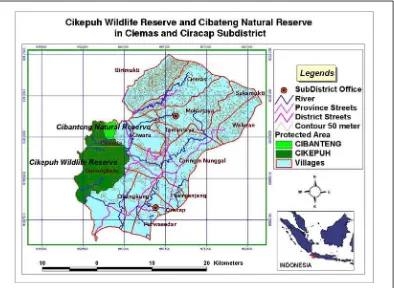
Figure 3.1. Study area, is included Ciemas and Ciracap Subdistrict of Sukabumi Province
17
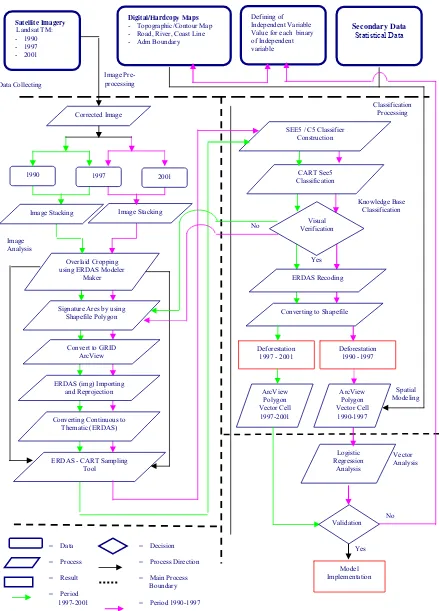
Figure 3.2. Flow chart of research activities and procedures 20
Figure 4.1. Stacking process of Landsat image 1990 and 1997 32
Figure 4.2. Defining a training site with one polygon and inside that polygon must be similar the spectral characteristic in both dates
33
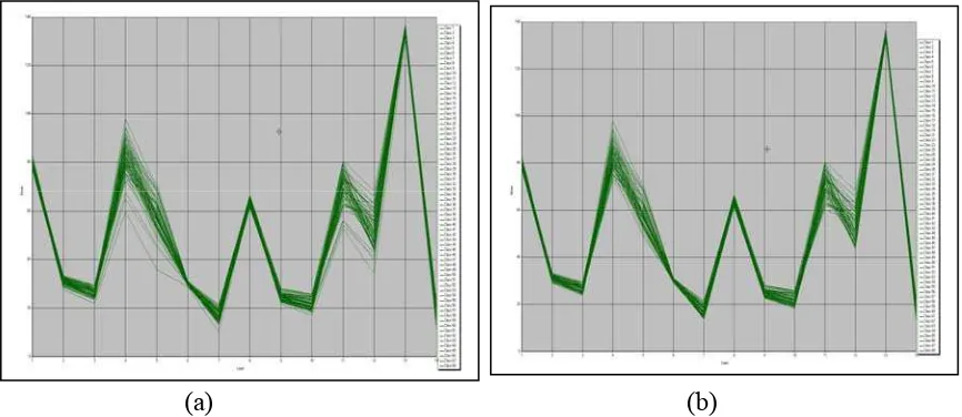
Figure 4.3. Observing the one class of stable forest by signature mean plot, which is similarity of spectral characteristic
34
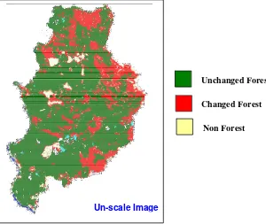
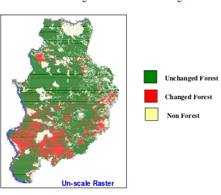
Figure 4.4. The result of classification process that is using ERDAS Imagine 8.7, CART and See5 for period 1990 - 1997
37
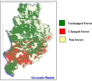
Figure 4.5. The result of classification process that is using ERDAS Imagine 8.7, CART and See5 for period 1997 - 2001
38
Figure 4.6. ERDAS Imagine 8.7 Modeler Maker, the model is to clip deforestation class in first period to the raster in second period.
39
Figure 4.7. The result of clipping process between deforestation class in Period 1990 -1997 will be as non-forest in Period 1997 – 2001.
39
Figure 4.8. The result of clipping process between boundary polygon of study area and square shaped of cells.
40
Figure 4.9. SRTM (Shuttle Radar Topography Mission) data of topography was obtained from GLCF website, and displaying by ERDAS Imagine 8.7
42
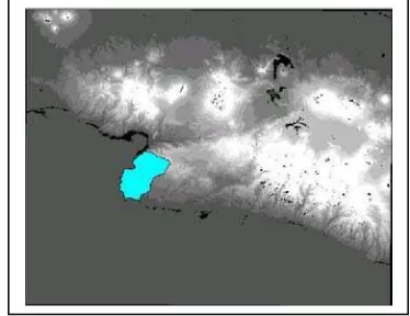
Figure 4.10. The result of assigning data by location (spatial join) of contour or altitude data (LogR_Alt), Figure 4.14. where yellow cells is altitude < 250 m (1) and light blue is ≥250 m (0).
42
Figure 4.11. The result of assigning data by location (spatial join) of river buffer (LogR_Riv) 1,000 m, where yellow cells is river or group of river < 1,000 m (1) and light blue is ≥ 1,000 m (0).
Figure 4.12. The result of assigning data by location (spatial join) of road buffer (LogR_Road) 1,000 m, where yellow cells is road or group of road network < 1,000 m (1) and light blue is ≥ 1,000 m (0)
45
Figure 4.13. The result of assigning data by location (spatial join) of shore line (LogR_SL) 1,000 m, where yellow cells is shoreline buffered < 1,000 m (1) and light blue is ≥ 1,000 m (0)
46
Figure 4.14. The result of assigning data by location (spatial join) of shore line (LogR_CP) 1,000 m, where yellow cells is center population buffered < 10,000 m (1) and light blue is ≥ 10,000 m (0)
47
Figure 4.15. The result of assigning data by location (spatial join) of aspect (LogR_COM), where yellow cells is East, West,, and flat area and remaining compass is the light blue.
49
Figure 4.16. The result of assigning data by location (spatial join) of slope (LogR_Slp), where yellow cells less 25 degree and the blue light is 25 – 90 degree.
50
Figure 4.17. Classification plot (ClassPlot), another very useful piece of information for assessing goodness of fit for the model
60
Figure 4.18. Comparison between prediction deforestation and actual deforestation in 2001.
LIST OF TABLE
No. Caption Page
Table 2.1 References of Regression logistic method for prediction model. 5
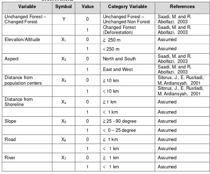
Table 3.1 Binary data and categorization of variables as the factors of deforestation ……… 27
Table 3.2 Recapitulation table as the result of SPSS calculation of logistic regression ……… 30
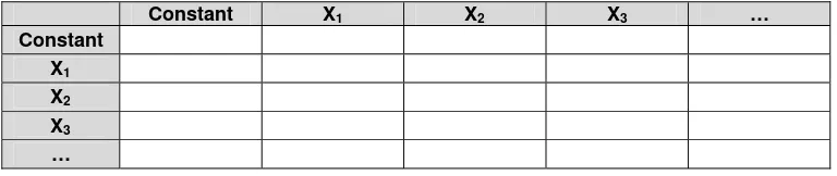
Table 3.3. Correlation matrix, that defining the correlation among the variables ……….. 30
Table 4.1 Variables not in the Equation ……….. 52
Table 4.2 Variables in the equation ……….. 53
Table 4.3 Variables in the Equation of null model ……….. 54
Table 4.4 Omnibus Tests of Model Coefficients ……… 54
Table 4.5 Hosmer and Lemeshow Test. ……….. 55
Table 4.6 Contingency Table for Hosmer and Lemeshow Test …………... 55
Table 4.7 Classification Table ………. 56
Table 4.8 Variables in the Equation and Wald test ……….. 58
Table 4.9 Recapitulation of raster classification process ………. 62
Table 4.10 Recapitulation of polygon vector cell process ………. 63
Table 4.11 Error matrix resulting from classifying logistic regression model ………..
LIST OF APPENDIX
No Caption Page
Appendix 1. Vector Map of Study Area ……… 74
Appendix 2. Illustration of attribute table in spatial processing ……… 75
Appendix 3. SPSS Output ……… 76
I. INTRODUCTION
1.1. Background
Wildlife reserve is a kind of protected area that possesses the unique
characteristic species and or biodiversity and to manage the habitat for their
living sustainability (Act (UU) No 5, 1990). Cikepuh Wildlife Reserve is
one of conservation area located in the southern of Sukabumi District, West
Java Province. Cikepuh Wildlife Reserve is bordered in the northern by
Cibanteng Natural Reserve. Cibanteng Natural Reserve is forest and natural
grass land and suitable for wildlife habitat.
Cikepuh Wildlife Reserve and Cibanteng Natural Reserve, since both
conservation area was established in 1973 and 1925 have been faced complex
problem caused by land use changed, deforestation, illegal hunting, forest
fire, and so on. Sahardjo (2000) indicated that Cikepuh Wildlife Reserve had
suffered from degradation forest, reaching 80%. Most of this degradation has
been caused by illegal logging for wood and paddy field. Deforestation itself
is a complex socio-economic, cultural, and political event. Concern over the
rate of deforestation has given rise to a literature that quantifies the impact of
forces that drive deforestation. The literature has focused on two questions:
(1) What factor affect the location of deforestation? And (2) What factors
affect the rate of deforestation? It is clearly important to know where
deforestation is likely to occur (Cropper, Puri, Griffiths 2001).
This thesis focused on the first question above by considering some
common driving forces of deforestation and using a spatial model to look at
broader condition and logistic regression model is proposed as an effective
framework for the modeling prediction of forest cover and non-forest
category associated with the spatial pattern and rates of deforestation.
Logistic regression model is a special type of regression models,
which used to study the probability of membership in two contradictory
identically such as deforestation possibility or stable forest. In the application
of logistic regression, each “observation” is a cell.
Recent development of GIS (Geographic Information System)
technology enhances the analytical power needed for the study of land use
and land cover change. Remote sensing is a science that records and analyses
the radiation reflected or emitted by the objects on the earth surface. The
nature of the object land cover type (forest) determines which proportion of
the radiation in a specific part of the electromagnetic spectrum (different
wavelength) will be reflected and recorded by sensor of the satellite. The
changes of land use and land cover due to natural and human activities can be
observed using current and historical remotely sensed data available form
archives.
1.2. Objectives
The objective of this study is to translate the complexity of
deforestation processes into simple model by using the statistical method of
logistic regression model which analyze the probability of deforestation in
each single cell. The purpose of this analysis is to measure the possibilities of
changed forest (deforestation) or unchanged forest based on the predictor or
variable factor of its driving force, such as distance from center of dweller,
aspect, slope, distance from shore line, distance from existing road, and
elevation.
As the main objective of this study is to observe the performance of
logistic regression model and spatial method, and the specific objectives are:
1. to quantify the forest cover and deforestation.
3. to elaborate spatial projection of future deforestation trends based
on possibility of deforestation resulted from predicting logistic
regression.
1.3. Hypothesis
Logistic regression does not assume a linear relationship between the
dependents and the independents variables. Logistic regression does not
require linear relationships between the independent variables as well, so in
this study the hypothesis for the logistic regression analysis will be:
At least one of independent variables such as distance from river road, shore
line and center of population, altitude, aspect, or slope is not equal to zero,
and can be used for predicting deforestation by the equation of logistic
II. LITERATURE REVIEW
2.1. Logistic Regression Model
Model can be interpreted as simplification of a system. While system
is the illustration of a process or some processes (some sub-system) regularly.
Model only depicting some aspects from a system and not have to express
entire process that happened in the system. More process that being
explained, the model will be more complex beside more inputs required. By
the reason, primary factors at one particular model are the target of when that
model is created. Based on the goal/target, model can be divided to become
three kinds of (1) to the understanding of process, (2) prediction, and (3) for
management purpose (Handoko 1994).
There are two distinct approaches to the modeling of systems: (1)
statistical models and (2) structural models. In statistical model, a relationship
between observed output and known input of a system is established by
postulating a general mating the parameter of the relationship by adjusting
them to best fit the empirical data. Regression and correlation analysis are
examples of this widely used method. While structural model attempt to
describe the structure of the system, which is responsible for its behavior
(Bossol 1986)
Logistic regression model is being used to analyze the relationship
between the explanatory variables and the outcome/response. The outcome
variable is categorized to be success or failure, i.e zero or one. It is assumed
each observation is independent one another, so that the number of success
events will be binomial distribution (Sutisna 2002). Also logistic regression
is a technique which used to analyzed data that its response variable is binary
or dichotomy scale (Hosmer and Lemeshow 1989 in Amanati 2001), and
independent variable can be continue or categorical-scale of data (Amanati
2001)
According to Saadi and Abolfazi (2003) that a logistic regression
model is a statistical model which a relation between a phenomenon (a
defined based on some observation. These observations are in fact a set of
values measured or observed for the dependent and independent variables.
Having the model specified and calibrated, the unknown value of the
phenomenon can be calculated and predicted on the basis of known values of
its factors.
Often, the spatial phenomenon under investigation can only be
described by a categorical variable for example bird distribution indicating
presence or absence of birds (Anonim 2004) or forest area being either
stables or destroy (Saadi and Abolfazi 2003). Another word according to
Saadi and Abolfazi (2003) mentioned that a regression model was a special
type of regression models, which used to study the probability of membership
in two contradictory classes. It should be noted that logistic regression can
be used to determine the probability of any of the two possibilities
(categories) identically. Previous regression technique is not suitable because
the dependent variable is neither interval or ratio (Anonim 2004).
Table 2.1 shows the references of logistic regression model that being
used to predict deforestation and other purposes.
Table 2.1. References of Regression logistic method for prediction model.
No Authors Research Title Methods Results
1
Chengling Xie Bo Huang
Christophe Claramunt Magesh Chnadramouli
Spatial logistic regression and GIS to model rural-urban land conversion
Log.Regression, GIS and Remote Sensing
Accuracy of correct prediction for developed area is 45.33 with overall accuracy 76.15%
2 Laura C. Schneider and R. Gil Pontius Jr.
Modeling land-use change in Ipswich watershed, Massachusetts,
Analysis and estimation of
deforestation using satellite imagery and GIS
Log.Regression, GIS and Remote Sensing
31.93 correctly predicted as unchanged pixels and 93.90% for changed
4 S. Lee
Cross-verification of spatial logistic regression for landslide
susceptibility analysis: A case study Korea lahan pada daerah Merang dengan menggunakan metode regresi logistic (Simulation of landuse change in Merang area by using
Log.Regression, GIS and Remote Sensing
2.1.1. Logistic Regression Equation
According to Scheider and Pontius Jr (2001) in their research
in Ipswich watershed, Massachusetts, USA, that in the application of
logistic regression, each “observation” is a grid cell. The dependent
variable is a binary presence or absence event, where 1 = changed
forest (deforestation) and 0 = unchanged forest or non-forest, for a
certain period of time. The logistic function gives the probability of
deforestation as a function of explanatory variables. The function is a
monotonic curvilinear response bounded between 0 and 1, given by a
logistic function of the form:
)
expected value (mean) of the binary dependent variable Y, β0 aconstant to be estimated, βi a coeficient to be estimated for each
independent variable Xi (where i = 1,2,3, …, p).
The logistic function can be transformed into a linear response with
the transformation :
⎟
The transformation (Eq. (2)) from the curvilinear response (Eq.
(1)) to linear function (Eq. (3)) is called a logit or logistic
transformation. The transformed function allows linear regression to
estimate each βi. Since each of the observations is a cell, the final
result is a probability score (p) for each cell (Scheider and Pontius Jr.
Model parameter can be estimated by an predictor maximum
likelihood, iterative reweighted least squares, and discriminant
analysis (Hosmer and Lemeshow 1989 in Amanati, 2001). Parameters
testing of logistic regression is based on assumption that parameter βi
is normal distributed (Freeman 1987 in Amanati 2001). In this study
maximum likelihood method is used to estimate the parameters βi.
2.1.2. Significance Tests for Parameter Predictor
There are numerous models in logistic regression: a constant
(intercept) only that includes no predictors (null model), an
incomplete model that includes the constant plus some predictors, a
full model that includes the constant plus all predictors, and a perfect
(hypothetical) model that would provide an exact fit of expected
frequencies to observe frequencies if only the right set of predictors
were measured (Tabachnick and Fidell 2001)
In SPSS program, there are two steps (model) as default. The
first step, called Step 0, includes no predictors and just the intercept,
and also called null model. And the second is the first step (or model)
with predictors in it. In this case, it is the full model that we specified
in the logistic regression command.
When it has no reasons for assigning some predictors higher
priority than others, statistical criteria can be used to determine order
in preliminary research. That is, if being wanted a reduce set of
predictors but has no preferences among them, stepwise method can
be used to reduced set (Tabachnick and Fedell 2001)
In this study, it uses Forward Stepwise of Maximum
Likelihood method in SPSS process, to obtain the statistical reasons.
SPSS allows to have different steps in a logistic regression model.
The difference between the steps is the predictors that are included.
begins with a full model and variables are eliminated from the model
in an iterative process. The fit of the model is tested after the
elimination of each variable to ensure that the model still adequately
fits the data. When no more variables can be eliminated from the
model, the analysis has been completed
Estimating parameter β0, β1, …, βp in the logistic regression
model, it can be done using maximum likelihood method. The
function of the model is given by : (Sutisna 2002)
For simply, the likelihood function can be written in the form of
log-likelihood as follow:
Once an adequate model has been obtained, the next step is to
test the significant of the parameter estimates. There are two types of
test that can be used, G-test, a likelihood ratio-based tests statistic and
Wald test.
G-test is used to test the significance all of the parameters in
the model. The formula of G statistic:
where Lo = likelihood without independent variable
Lp = likelihood with independent variable
with hypothesis of test:
H0 = β0 = β1 = β2 = β3 = … = βp = 0
Under the null hypothesis H0 the G-statistic will follow a
chi-square distribution with p degree of freedom (Hosmer and Lemeshow
1989 in Sutisna 2002), so a chi-square test is the test of the fit of the
model
Wald test is used to test the significance of parameter βi,
where i = 1,2,3, .., p partially. This test is used, when the null
hypothesis H0 in the G-statistic is rejected. The formula of Wald test:
With βˆi is the estimator for coefficient βi and SE
( )
βˆi is thestandard error of . Null hypothesis for coefficient regression is zero
will be rejected if |W
i
βˆ
i| > Wα/2. Under the null hypothesis the Wald test
will follow normal distribution (Hosmer and Lemeshow, 1989 in
Sutisna 2002).
2.1.3. Model Interpretation
SPSS will offer a variety of statistical tests. Usually, though,
overall significance is tested using what SPSS calls the Model Chi
-square, which is derived from the likelihood of observing the actual
data under the assumption that the model that has been fitted is
accurate. It is convenient to use -2 times the log (base e) of this
likelihood; it’s called -2LL. The difference between -2LL for the
best-fitting model (full model) and -2LL (null model) for the null
hypothesis model – initial chi-square (in which all the β values are set
to zero) is distributed like chi-squared, with degrees of freedom equal
to the number of predictors; this difference is the Model chi-square
that SPSS refers to. Very conveniently, the difference between -2LL
values for models with successive terms added also has a chi-squared
distribution, so when using a stepwise procedure, it can use
significantly improves the fit of our model (Departement of
Psychology–University of Exeter 1997).
Model chi-square measures the improvement in fit that the
explanatory variables make compared to the null model. Model
chi-square is a likelihood ratio test which reflects the difference between
error not knowing the independents (initial chi-square) and error when
the independents are included in the model (deviance). When
probability (model chi-square) ≤ .05, it reject the null hypothesis that
knowing the independents makes no difference in predicting the
dependent in logistic regression (CHASS-NCSU 2006).
Coefficient of logit model can be formulated as βI = g (x+1) –
g(x). Parameter of βi, depicts the change of g(x) logit function for the
changing of one unit of independent variable x, and as called log odds
(Hosmer and Lemeshow 1989 in Amanati 2001).
For significance of individual predictors, SPSS also offer what
it calls Wald statistic, together with a corresponding significant level.
The Wald statistic also has a chi-squared distribution (Departement of
Psychology – University of Exeter 1997).
The ratio of the logistic coefficient β to is Standard Error (SE)
squared, equals the Wald statistic. If the Wald statistic is significant
(i.e less than 0.05) then the parameter is significant in the model.
Coefficient interpretation its self will be done for the significant
predictors by seeing the value of each coefficient. If the coefficient is
positive, it tends Y =1 to be greater than for occurring independent
variable X = 1 than X = 0.
According to Hosmer and Lemeshow (1989) in Amanati
independent variable X that call Odd Ratio. Log odds is difference
between two values of logit, and being noted as:
ln [ψ (a,b)] = g(x=a) – g(x=b)
= βi (a-b)
One of the values of risk level is odd ratio (Freeman 1987 in
Amanati 2001). For dichotomy variables, the estimator of odds ratio
is:
ψ = [π(1) / (1- π(1))] / [π(0) / (1- π(0))] ln (ψ) = g(1) – g(0)
ln (ψ) = βi
ψ = exp [βi (1-0)]
With the result that, if a-b=1, so ψ = exp(βi). This odd ratio can be
interpreted as a tendency of Y=1 at x = 1 with the amount of ψtimes by comparing at x = 0 (Amanati 2001).
2.1.4. Logistic coefficients and correlation
Note that a logistic coefficient may be found to be significant
when the corresponding correlation is found to be not significant, and
vice versa. To make certain global statements about the significance
of an independent variable, both the correlation and the logit should be
significant. Among the reasons why correlations and logistic
coefficients may differ in significance are these: (1) logistic
coefficients are partial coefficients, controlling for other variables in
the model, whereas correlation coefficients are uncontrolled; (2)
logistic coefficients reflect linear and nonlinear relationships, whereas
correlation reflects only linear relationships; and (3) a significant logit
means there is a relation of the independent variable to the dependent
variable for selected control groups, but not necessarily overall
(College of Humanities & Social Sciences, North Carolina State
2.2. Remote Sensing, GIS and Change Detection 2.2.1. Remote Sensing
Remote sensing is the science and art of obtaining information
about an object, area, or phenomenon through the analysis of data
acquired by a device that have no any contact with the object, area, or
phenomenon investigated (Lillesand and Kiefer 2000).
Remote sensing is the instrumentation, techniques and methods
to observe the Earth’s surface at a distance and to interpret the images
or numerical values obtained in order to acquired meaningful
information of particular object on Earth (Buiten and Clevers 1993).
Before the image data can produce the required the information
about the objects or phenomenon of interest, they need to be
processed. The analysis and information extraction or information
production is a part or overall remote sensing process, known as
image processing. Digital image processing involves the
manipulation and interpretation of digital image with the aid of a
computer and a certain program or software.
The central idea image behind digital image processing is quite
simple. The digital image is fed into computer one pixel at a time.
The computer is programmed to insert these data into an equation, or
series of questions, and then store the results of the computation for
each pixel. These results form a new digital image that may be
displayed or recorded in pictorial format may itself be further
manipulated by additional programs (Lillesand and Kiefer 2000).
2.2.2. Change Detection
Change detection is the process of identifying differences in
the state of an object or phenomenon by observing it in different
times. The basic premise in using remote sensing data for change
in radiance values or local texture that are separable from changes
caused by other factors, such as differences in atmospheric conditions,
illumination and viewing angle, soil moisture, etc. It may further be
necessary to require that changes of interest be separable from
expected or uninteresting events, such as seasonal, weather, tidal or
diurnal effects. Some techniques also assume that the areas of change
will be relatively small (Deer 2004).
2.2.3. Geographical Information System
A geographic information or Geographic Information System
(GIS) is a system for creating, storing, analyzing and managing spatial
data and associated attributes. In the strictest sense, it is a computer
system capable of integrating, storing, editing, analyzing, sharing, and
displaying geographically-referenced information.
(http://en.wikipedia.org/wiki/Geographic_information_system).
GIS depicts the real world through model involving geometry
(spatial information), attributes, relation, and data quality. Spatial
information is presented in two ways: as vector data in the form of
points, lines, and areas (polygons) or as grid data in the form of
uniform, systematically organized cell (raster) ( Bernhardsen 1992).
All geographic phenomenon have various relationships among
each other and possess spatial (geometric), thematic and temporal
attributes (de By 2000). Phenomenon are classified into thematic data
layers depending on the purpose of database as for example land use
data layers that can be analyzed (spatial analysis) involves question
about data that relate topological and other relationship. Such
question may involve neighborhood, distance, and few more
characteristics that may exist among geographic phenomenon (de By
2000). So that in the attributes data that relates with spatial data can
be manipulated, added, eliminated, and so on, for example in the
regression logistic. This condition, is especially for discrete grid/cell
data that can be analyzed further from each cell for any purposes.
2.3. Deforestation
Forest decline is interpreted as deforestation, forest degradation or a
combination of both. The Food and Agricultural Organization of the United
Nations defines deforestation as the “sum of all transitions from natural forest
classes (continuous and fragmented) to all other classes” (FAO 2006). The
loss of forest cover attributed to these transitions must occur over less than
10% of the crown cover for the phenomenon to quality as deforestation
(Contreras-Hermosilla 2000).
In addition to deforestation, forest degradation is an issues. According
to FAO, changes within a forest class, for example for closed to open forest,
which negatively affect the stands or, in particular, lower its production
capacity, constitute forest degradation. Thus, forest degradation implies a
major loss of forest productive capacity, even where there is little
deforestation as such.
In this thesis deforestation is the forest decline, forest loss from one
period of time without considering the reduction of tree crown cover less
than 10% of total area for rather large areas and for long period of time and
will not attempt a rigorous definition of “large area” and “long period of
time”.
According to the World Resources Institute, the world has lost about
half of its forest cover. Despite a number of initiatives to stop forest decline,
the world continues to lose some 15 million hectares of forest every year.
Deforestation over the period 1980-1999 reached 8.2% of total forest area in
Asia. Most modern deforestation takes place in developing countries,
According to FWI/GFW (2001), actually Indonesia still has close
forest in the year 1950. About 40 percentage of forest areas in the year 1950
have been cut away during 50 next year. If rounded up, forest cover in
Indonesia have decreased from 162 million ha become 98 million ha. Rate of
forest losing is increasing progressively. In the year 1980-an accelerating
losing of forest in Indonesia mean about 1 million ha per year, later increase
to become about 1,7 million ha per year at first years of 1990. Since year
1996, accelerating deforestation seems re-increasing to become mean 2
million ha per year.
Although Java Island contributes only about 7% of total land in
Indonesia (MOF and FAO 1990), but it is unique because of its high
population and intensive agriculture (Verburg, Veldkamp, Bouma 1999).
And they contain over 60% of the population and produce some two-third of
the country’s food supplies (Verburg, Veldkamp, and Bouma 1999).
Demography transition and growth of economics in Java Island where
possesses population about 132 million people, have caused expanding of
agriculture and wide of forest degradation from time to time. Obtained
information has shown that from 16th century until mid of 18th century,
natural forest in Java about 9 million ha. To the last year 1980th, natural
forest cover in Java only reaching 0.96 million ha or 7% from Java land
(Kartodihardjo et al. 2003).
Encroachment and deforestation in Cikepuh Wildlife Reserve,
according to Eddy (2004) was aimed to change the land function into
settlement and fixed cultivation, and almost half of total wide of Cikepuh
Wildlife Reserve.
With regard to policy issues, the problem with deforestation policy in
Indonesia in general is not so much the policy logging, but the conversion of
land to other uses, where the other uses have no economic potential. This
policy is implicated in leading to unsustainable activities and resulting in land
III. RESEARCH METHODOLOGY
3.1. Time and Location
The research would require six months, it had started from December
2004 to May 2005, from problem identification, finding related references to
writing research proposal. It remains the processing, analyzing data and
discussing the result.
The study area had been carried out place in Sukabumi province, and
only two districts will be chosen as the unit of sub-district: Ciemas and
Ciracap. Nature Preserve (Cagar Alam) Cibanteng and Wildlife Reserve
(Suaka Margasatwa) Citepuh are inside both two subdistrict. These
conservation areas will be study area. The ecosystem inside, there are low
land forest and sub-mountain forest, and bounded by Indonesia Ocean, so that
coastal ecosystem included.
The area is assumed that no organized illegal logging in large scale,
only community in two districts and surrounding forest interact with the
forest condition. The location is about 120 km far from Province Capital City
of Sukabumi and about 240 km from Jakarta.
Geographically, the both districts area is about 0 – 1000 m from sea
level (BPS 2000), bounded by longitudes 106o 20' - 106o 40' and latitudes
7o 05' - 7o 30'. The area of Ciemas Subdistrict is about 26,696 ha and Ciracap
Subdistrict about 22,237.44 ha (BPS 1996)
The borders of that area are:
1. Northern part is adjacent to Pelabuhan Ratu and Lengkong Subdistrict.
2. West part is adjacent to Indonesia Ocean.
3. South part is adjacent to Indonesia Ocean.
In this research, the spatial analysis processing for both subdistricts
are treated as the administration unit, but Cikepuh Wildlife Reserve and
Cibanteng Natural Reserve had been treated as a study area and combined
into one focus area. Map of the study area can be seen in Figure 3.1 and
more detail in Appendix I
Figure 3.1. Study area, is included Ciemas and Ciracap Subdistrict of Sukabumi Province
3.2. Data Sources
Data required to support this research, included:
(1). Satellite imagery, from data Landsat TM with series data (multi-date),
covering Districts of Ciemas and Ciracap. The path/row image is
122/65, acquisition date Nov. 9th, 1990, July 28th, 1997, received from
PPLH (Pusat Penelitian Lingkungan Hidup / Environmental Research
and May,12th 2001 downloaded from GLCF (Global Land Cover
Facility) (http://glcf.umiacs.umd.edu/index.shtml)
(2). Topographic Map is obtained from SRTM (Shuttle Radar Topographic
Mission) format and downloaded from GLCF (Global Land Cover
Facility) (http://glcf.umiacs.umd.edu/index.shtml) with acquisition data
2000
(3). Digital Map of Village, Sub-district, was received from PPLH-IPB, in
vector or shp format
(4). Digital Map of Nature Preserve (Cagar Alam) Cibanteng and Wildlife
Reserve (Suaka Margasatwa) Citepuh boundary, was received from
Baplan (Badan Planologi / Forestry Planning Agency) Ministry of
Forestry.
(5). Demographic and socio-economic data, which is collected from BPS
(Badan Pusat Statistik / Bureau of Statistical Center) Sukabumi
Province and Head Office Jakarta.
3.3. Supporting Tools/Program
In this research, supporting tools used, as the terms of software and
hardware are as the followings:
(1). Software:
• ERDAS Imagine 8.7 used for image processing
• ArcView 3.3, used for spatial data processing
• See5 (C5) Ver. 2, used for classification process and combined with ERDAS Imagine.
• SPSS version 11.5, used for statistical calculation and analysis.
(2). Hardware:
• PC Dual Processor Xeon™ Intel® Pentium® IV CPU 2.99 GHZ, 1 Gb DDR-SDRAM, Video System NVIDIA GeForce 6600 256 Mb, working at Operating System Window XP Service Pack 2
3.4. Methodology
On the whole of research procedure will be illustrated in Figure 3.2.
3.4.1. Image Preprocessing
The objectives of image preprocessing are to remove some
error because of the radiance measured by any given system over a
given object on earth surface is influenced by such factors as changes
in scene illumination, atmospheric conditions, viewing geometry, and
instrument response characteristics.
(a) Radiometric/Atmospheric Correction. Histogram Adjustment is one of method that can be used. Histogram adjustment is used
to minimize atmospheric bias. This process is common process
to pre image processing, but in this thesis this process was not
done since the ERDAS Imagine can accommodate to identify the
similarity of DN (Digital Number) value for each area of interest
for training sites or signatures area b using mean plot tool. Only
image enhancement method that will be done for improving the
visual interpretability in order to increase the apparent distinction
between the features in that Landsat scenes, such as contrast
stretching by standard deviation in ERDAS Imagine 8.7
(b) Geo-Referencing, raw digital image usually contain geometric distortions so significant that they can not be used directly as a
map base without subsequent processing. The sources of these
distortions range from variations in the altitude, attitude, latitude,
and velocity of the sensor platform to factors such as panoramic
distortion, earth curvature, atmospheric refraction, relief
displacement, and non-linearities in the sweep of a sensor’s
IFOV. The aim of geometric correction is to compensate for the
distortions introduced by these factors so that the corrected image
Knowledge Base - Road, River, Coast Line - Adm Boundary Signature Ares by using
Shapefile Polygon
ERDAS - CART Sampling Tool
CART See5 Classification
Converting to Shapefile
ArcView
SEE5 / C5 Classifier Construction Value for each binary ofIndependent variable
Random distortions and residual unknown systematic distortions
are corrected by analyzing well-distributed ground control points
(GCPs) occurring in an image. From another corrected-image,
GCPs are features of known ground location that can be
accurately located on the uncorrected image to become a new
corrected-image, also known as rectification process.
Actually this was not done in this research, the images
from GLCF just need to be projected to UTM Zone 48 South and
Datum WGS 84. In the process also was needed GCP (Ground
Control Points), it has about 30 points with first polynomial
order. A first order polynomial is normally suitable for a
transformation between two near recti-linear map systems.
Landsat images are from year 1995 and 1997 acquisition
are in bsq (binary sequential), so it needed to export bsq to img
(ERDAS format) with certain and fix number of rows and
columns. Image acquired in the year 2001, was treated as master,
and while the others 1990 and 1997 were referred to as slave
images.
3.4.2. Image Processing
The methodology of image processing in this research is using
classification method that obtained from CABS (Center for Applied
Biodiversity Science) CI (Conservation International) Washington
DC and developed together with Wildlife Conservation Society
(WCS) – Indonesia Program. In this method, the classification uses
CART tool as one of ERDAS Imagine 8.7 plug in and stand alone
program See5 (C5), as the additional program to support better
classification.
122065_19901109_ 19970728 . This stacked-image is called
Period 1990-1997. Period 1997 – 2001 that will be used for
validating, was done with the same procedure to stack the images
122065_19970728 with 122065_ 20010512 became
122065_19970728_20010512.
This stacking process always has remaining edge as the result of
process, since the wide of both images are not same. This edge
must be cut by using ERDAS Imagine Modeler Maker
(b) Signature areas, to obtain the interest area was done by cropping Ciemas and Ciracap Subdistrict based on digital administrative
boundary data, with the same projection, and the last
subset/cropping again to obtained both conservation area Nature
Reserve (Cagar Alam) Cibanteng and Wildlife Reserve (Suaka
Margasatwa) Cikepuh as the study area. Signature areas or
training sites are used to define a certain class based on
visualization characteristic. Signature area was made in polygons
shapefile format in ERDAS Imagine 8.7. Start to take a signature
area or training site is to zoom the interest area and make one
representative polygon that make sure the characteristic spectral
inside that polygon is similar whether first date
(1220065_19901109) has one class for instant forest and the
second date (122065_19970728) also has one class for instant
non-forest. So the entire signature areas is stand alone layer in
vector format in ERDAS Imagine 8.7
In this study, 5 main land cover categories were distinguished:
- Forest, to identify forest that no change to another uses.
- Non-Forest, assumed as agriculture area, plantation, settlement,
shrub or bush, bare land, and even seasonal flooding
- Cloud, but in the thesis, the land use or land cover will be
estimated with the surround condition.
- Shadow, in the thesis, the land use or land cover will be estimated
with the surround condition, since binomial logistic regression can
not use cloud and shadow class. So water, cloud and shadow, at
the last process will be included as non-forest category, if the cloud
and shadow are among the non-forest area category
ID of each signature area polygon in shapefile format as
attributes is one important thing to recode and classify the image.
Two digits can be used for 8 bits of classification result and 4
digits for unsigned 16 bits. Four digits will be more to determine
as many as classes in order to minimize DN (Digital Number )
overlapping for each class.
Note field is just for describing the ID, example for making one
particular a forest class to differ with the others by visualization
interpretation. The forest says swamp forest, according to the
class that we want to extract only forest and non-forest, and
because of this fact we make particular ID for example start from
1140, 1141, and so on. At the last process, after getting the best
iteration, the image must be converted again to 8 bit data type
and recode to common classes forest to forest (11), forest to non
(12), non to non (22), water (44), cloud (55), and shadow (66).
As mentioned before, that it is better to use 16 bits output data
type, to anticipate overlapping amount training sites, one training
site will represent one type of spectral characteristic. In this case,
forest class was collected, and numbered with 4 digits. After
obtaining all spectral characteristic of forest, it needs to verify the
similarity of forest spectral characteristic. This task can be done
by using Mean Plot of Signature in ERDAS Imagine 8.7. So the
areas which have had similarity of spectral characteristic.
However this technique is only for unchanged class such as
forest to forest, and can not be used for changed forest to non,
because non forest class in this case may be depicted many land
cover for example seasonal flooding, mixed agricultural or
farming, plantation, and so on.
Mean plot of signature is a spectral profile of the mean data file
value of each signature in all bands of the image to be classified
was obtained by changing the polygon in shapefile format to
AOI. It uses Copy Selection to AOI, from AOI menu in ERDAS
Imagine 8.7 Viewer. After all classes assumed are right, the
polygon shapefile will be converted to grid by using ArcView
3.3.
ArcView program is used for converting shapefile of signature
areas polygon into grid format. This grid must be same the pixel
size. Using ERDAS Imagine again is to import the Grid type
into img format, with data type unsigned 16 bit in Import
Options. Open one ERDAS Imagine viewer again to see the
result of importing process. In this process, the projection
metadata will loose, and it needs to be redefined. From ERDAS
Image Information, change the Map Model, the unit into meters
and projection into UTM (Universal Transfer Mercator) and
change Spheroid and Datum WGS 84, UTM Zone 48 South.
The result of above process is still continuous file type, and it
must in thematic file type. This process uses Modeler Maker,
and the model will change continuous to thematic file type, with
the same data type 16 bit.
(c) ERDAS Imagine – CART Classification. Classification process uses CART, from ERDAS tool bar, and choose CART Sampling
Dependent Variable File is thematic img file after converting
process, uses See5, and the last define the third file output
*.names, *.data, and *.test.
After that, process is continued by using stand alone program
See5. From See5 main menu, choose File – Locate Data, and find
the path of *.data as the result of CART Sampling Tool. Choose
File – Construct Classifier, and CC Option window will appear,
check list Boost with 10 default value and the remaining let them
as default value, Pruning CF 10% and Minimum 2 Cases in
Global Pruning option.
See5 will run the classification process according to the dependent
and independent variable files. If the See5 process is success, the
last classification process is to appear the thematic image. Back
to ERDAS Imagine tool bar menu, choose CART again and click
Run See5.
Run See5 in submenu CART tool in ERDAS is the last process of
classification. The result can be interpreted to the original image,
and if there are many mistaken, it can be iterated and so on.
Iteration starts at defining the signature areas polygon again, and
continue the process. This result also can be used to further
process, to convert to vector format. Since until this process, data
type 16 bit still inside, the raster must be converted again to 8 bit,
in order to be easy to further process. The class ID in the raster
attribute data must be 11, 12, 22, 44, 55, or 66. Recoding of
ERDAS Imagine 8.7 is needed in this case.
Period 1997 – 2001 will be done by the same procedure. Image
data 1997 is the same date with image data in period 1990 – 1997,
it is 122065_19901109 and 122065_20010512 for image data
In this case, with the assumption that deforestation in Period 1990
– 1997 will be non-forest in Period 1997 – 2001, since the image
data 1997 will be the first date and image 2001 will be the second
date. Both images became one stacked image. By the reason, the
deforestation class (class number 12) will be clipped by all classes
of raster Period 1990 – 1997. Only class number 12 of Period
1997 – 2001 will be as input theme and Period 1990 – 1997 will
be as clip theme. This process is done by using Modeler Maker
ERDAS Imagine 8.7
3.4.3. Vector Processing
(a) Creating Cell Vector, In this study as the nest for attribute data of each variables is cells. The cell is polygon with square shape,
with size 90 x 90 meters. These vector cells were created by
using ET Vector Grid, a plug in extension of ArcView 3.3. In its
process, this tool just need four input extents points, Xmin, Xmax,
Ymin, and Ymax; and XY spacing or grid resolution 90 meters.
The result of this process is a squared shape, which consist of cells
or grids.
Each cell has to be filled by either value 0 or 1 for independent
and dependent variables. Joining process to fill each cell, will be easy by using ArcView Extension, Geoprocessing Assign data by
location (Spatial Join). The tool will join the ID of cell correlated
by either value 0 or 1, in an attribute table, and was saved by a
name Polygon VectorCell (PVC). Name of PVC is based on ArcView extension to create grid vector polygon, and to differ
with raster grid in this thesis, grid is changed to cell. The results
process are spatial and its attributes, that must be saved into a new
(b) Extracting Variables Data
In this research, dependent variable and independent variable will
be list in Table 3.1.
Table 3.1. Binary data and categorization of variables as the factors of deforestation
Variable Symbol Value Category Variable References
Unchanged Forest –
Changed Forest Y 0
Unchanged Forest – Unchanged Non Forest
Sitorus, J., E. Rustiadi, M. Ardiansyah. 2001
1 < 10 km Sitorus, J., E. Rustiadi,
M. Ardiansyah. 2001 Distance from
Extracting vector data starts from obtaining the polygon that
contains the attribute data such as contour data ≥ 250 meters and <
250 meters. Sometimes this purpose needs editing manually of
using ArcView extension in order to make easy the process. The
binary data must be put into the Polygon Vector Cell as attribute
data by using Assign data by location (Spatial Join). It is done the
same thing to other variables: road, river, distance from
population center, and distance from shoreline. Independent
tends to occur deforestation. The references and research citation
is presented in Table 3.1.
In ArcView 3.3, there is an extension Edit Tool 3.5, can
accommodate the purpose. There are three method to assign the
data by location, i.e Inside (attribute of polygon source must be
inside of the polygon target), Center Inside (attribute of polygon
source must be touched the center point of polygon target, and
Intersect (attribute of polygon source must intersect to the polygon
target). This tool is the same with Geoprocessing extension
Assign Data by Location.
In order to anticipate over estimation of deforestation, the Inside
method is applied to this research.
The process of extracting slope and aspect are different with
others. Extracting both features are using ArcView 3D Analyst
for creating TIN from Features. The next process that uses grid
TIN is using ArcView ModelBuilder. ModelBuilder will identify
input automatically of grid theme, in this case the result from
gridding TIN file.
Extracting aspect from elevation grid file is provide default by
ArcView ModelBuilder. It will produce classification of aspect in
raster or grid format that also as thematic or discrete grid theme;
with defined resolution 90 meters. The grid classes are:
• 1 = Flat
• 2 = North
• 3 = Northeast
• 4 = East
• 5 = Southeast
• 6 = South
• 7 = Southwest
• 8 = West
With the same procedure above, slope can be extracted. Slope is
in degrees unit, meter for vertical unit and slope would be
classified into ten classes.
• 1 = 0 – 5 degree
• 2 = 5 – 10 degree
• 3 = 10 – 15 degree
• 4 = 15 – 20 degree
• 5 = 20 – 25 degree
• 6 = 25 – 30 degree
• 7 = 30 – 35 degree
• 8 = 35 – 40 degree
• 9 = 40 – 45 degree
• 10 = 45 – 90 degree
3.4.4. Logistic Regression Model
Logistic Regression Model, is used to determine the
probability of Unchanged Forest / Unchanged Non-forest and
Changed Forest (Deforestation) that will occur by using transformed
function of:
π’ = (β0 + β1 X1 + β2 X2 + … + βp Xp)
where: π’ = probability of dependent variable Changed Forest (Y)
β0 = constant of regression
β1 = coefficient of X1 independent variable
β2 = coefficient of X2 independent variable
βp = coefficient of pth of X independent variable
According to Saadi and Abolfazl (2003) that they used and
selected a sampling set about 5% of total pixels, but in this research,
sampling set will be obtained from all cells that are from the result of
classification result. The entire sampling set that entered into Polygon
Vector Cell attribute, will be processed calculation by SPSS
Statistical computer program. Both possibilities value of variables
been mentioned in Chapter II (Literature Review). The result of the
calculation will be recapitulated such Table 3.2.
Table 3.2. Recapitulation table as the result of SPSS calculation of logistic regression
β Standard Error Wald df (degree of freedom) Significant
level exp (β) Constant
X1 X2 X3 …
Beside calculating and printing the statistic of logistic regression
model, SPSS also can calculate the correlation among or inter the
variables, as the result correlation will be display in matrix form, such
Table 3.3.
Table 3.3. Correlation matrix, that defining the correlation among the variables
Constant X1 X2 X3 …
Constant X1 X2 X3 …
Between two variable will have correlation if the correlation value
more then or equal 0.5, and less then 0.5, there is no relationship
between them.
3.5. Assumption of Research
1. Supervised Classification by visual interpretation is assumed to be
2. Cloud, shadow, and water, will be included as the closest class around,
for example cloud and shadow that are inside the forest area category;
they will be included as forest class. Oppositely, if cloud an shadow are
among the non-forest category, they will be non-forest class. This
process is done by recode tool of ERDAS Imagine 8.7
3. As the consequence of assumption no.2 above, could, shadow, and
seasonal flooding are assumed as 0 value. Because of calculation
process, logistic regression can not identify value unless 1 and 0.
4. Road is class of sub district road that be able to be passed only by car
and truck, so only district and province street class are used in this study
5. Logistic regression does not assume a linear relationship between the
dependents and the independents.
6. The dependent variable doesn’t need not to normally distribution.
7. Vector data and projection result are assumed correctly.
8. Center of population is approached by subdistrict office as point feature
IV. RESULTS AND DISCUSSION
4.1. Image Processing
4.1.1. Period 1990 - 1997
Both image data of 122065_19901109 and
122065_19970728 have been stacked each other, became 14 (with
Thermal Band 6) bands/layers into one file of dataset
122065_19901109_19970728, and properly overlayed with the same
projection UTM (Universal Transverse Mercator) zone 48 South, and
Datum WGS 84.
This research image processing uses ERDAS Imagine 8.7,
from doing subset, geometric correction, until classification process.
The result of stacking process and the origin sources Landsat
images can be seen in Figure 4.1, with band combination 4-5-3 or
11-12-10.
Un-scale Image Un-scale Image
a. 1990 b. 1997
Getting the signatures area or training sites is done by using
polygon shape. Starting to take a signature area or training site, done
by zooming the interest area and make one representative polygon
that make sure the characteristic spectral inside that polygon is similar
whether first date (1220065_19901109) has one class for instant
forest and the second date (122065_19970728) also has one class for
instant non-forest (Figure 4.2). This class will be forest to forest area
or stable forest with class number 11.
Saving the training site as an attribute is one of the step, and
this attribute will be useful as the attribute in further vector process.
ID in attribute is one important thing to recode and classify the image
as well. Two digits can be used for 8 bits of classification result and 4
digits for unsigned 16 bits. Four digits will be more to determine as
many as classes in order to minimize DN (Digital Number)
overlapping for each class.
Un-scale Image
a. 1990 b. 1997
Another process in naming the polygon for each class name
is “note field”. Note field is just for describing the ID, for example is
to make one particular a forest class with different with the others by
visualization interpretation. The forest says dense forest, according to
the class that we want to extract only forest and non-forest, and
because of this fact we make particular ID for example start from
1140, 1141, and so on. Since in this classification using 16 bit data
type, class 11 (forest –forest) might be 100 subclass from 1100 to
1199.
The important part of classification process is to define the
signature area or training site. A training site must depict the entire
similar pixels. Pixels of cloud for instant can not include in a training
site of forest, although only one pixel (Figure 4.2).
It is better using 16 bits output data type rather than 8 bit, to
anticipate overlapping amount training sites, one training site will
represent one of spectral characteristic. In this case, forest class was
collected, and numbered with 4 digits, after obtaining all spectral
characteristic of forest, it needs to verify the similarity of forest
spectral characteristic. This task can be done by using mean plot of
signature in ERDAS Imagine (Figure 4.3).
(a) (b)