Introduction to Computational Science:
Modeling and Simulation for the Sciences, 2nd Edition Angela B. Shiflet and George W. Shiflet
Wofford College
© 2014 by Princeton University Press
Introduction
Modul 4 prepares you to use MATLAB for material in Chapter 9 and subsequent chapters.
Besides being a system with powerful commands, MATLAB is a programming language. In this tutorial, we consider some of the commands for the higher level
constructs selection and looping that are available in MATLAB. Besides more traditional applications, looping enables us to generate graphical animations that help in
visualization of concepts.
Random Numbers
Random numbers are essential for computer simulations of real-life events, such as weather or nuclear reactions. To pick the next weather or nuclear event, the computer generates a sequence of numbers, called random numbers or pseudorandom numbers. As we discuss in Module 9.2 , "Simulations," an algorithm actually produces the
numbers; so they are not really random, but they appear to be random. A uniform random number generator produces numbers in a uniform distribution with each number having an equal likelihood of being anywhere within a specified range. For example, suppose we wish to generate a sequence of uniformly distributed, four-digit random integers. The algorithm used to accomplish this should, in the long run, produce approximately as many numbers between, say, 1000 and 2000 as it does between 8000 and 9000.
Definition Pseudorandom numbers (also called random numbers) are a
sequence of numbers that an algorithm produces but which appear to be generated randomly. The sequence of random numbers is uniformly distributed if each random number has an equal likelihood of being anywhere within a specified range.
MATLAB provides the random number generator rand. Each call to rand returns a uniformly distributed pseudorandom floating point number between 0 and 1. Evaluate the following command several times to observe the generation of different random numbers:
rand
With one integer argument, rand(n) returns a square array with n rows and n
columns of random numbers between 0 and 1. Similarly, rand(m, n) returns an array with m rows and n columns of random numbers.
Suppose, however, we need a random floating point number from 0.0 up to 5.0. Because the length of this interval is 5.0, we multiply by this value (5.0 * rand) to stretch the interval of numbers. Mathematically we have the following:
0.0 ≤ rand < 1.0
Thus, multiplying by 5.0 throughout, we obtain the correct interval, as shown:
0.0 ≤ 5.0 * rand < 5.0
If the lower bound of the range is different from 0, we must also add that value. For example, if we need a random floating point number from 2.0 up to 7.0, we multiply by the length of the interval, 7.0 – 2.0 = 5.0, to expand the range. We then add the lower bound, 2.0, to shift or translate the result.
2.0 ≤ (7.0 – 2.0) * rand + 2.0 < 7.0
Generalizing, we can obtain a uniformly distributed floating point number from a up to b with the following computation:
(b - a) * rand + a
Quick Review Question 1 Start a new Script. In opening comments, have "MATLAB Tutorial 4 Answers" and your name. Save the file under the name
MATLABTutorial4Ans.m. In the file, preface this and all subsequent Quick Review Questions with a comment that has "%% QRQ" and the question number, such as follows:
%% QRQ 1 a
a. Generate a 3-by3 array of random floating point numbers between 0 and 1. b. Generate a 1-by-5 array of random floating point numbers between 0 and 10. c. Generate a 2-by-4 array of random floating point numbers between 8 and 12.
To obtain an integer random number, we use the randi function. The function call randi(imax) returns a random integer between 1 and imax, inclusively. Thus, the
following command returns a random integer from the set {1, 2, …, 25}:
randi(25)
For arrays we employ randi(imax, n) and randi(imax, m, n) to return n-by-n and m-by-n
arrays of random integers between 1 and imax, respectively. Thus, the following commands assign to matSqr a 4-by-4 array of integers from the set {1, 2, …, 25} and to
matRect a 2-by-3 array of integers from the same set:
matSqr = randi(25, 4)
matRect = randi(25, 2, 3)
Thus, to return a 2-by-3 array of integers in the set {0, 1, 2, …, 24}, we can employ the following command:
randi([0, 24], 2, 3)
Quick Review Question 2
a. Give the command to generate a number representing a random throw of a die with a return value of 1, 2, 3, 4, 5, or 6.
b. Give the command to generate a random number representing ages from 18 to 22, inclusively, that is, a random integer from the set {18, 19, 20, 21, 22}.
A random number generator starts with a number, which we call a seed because all subsequent random numbers sprout from it. The generator uses the seed in a computation to produce a pseudorandom number. The algorithm employs that value as the seed in the computation of the next random number, and so on.
Typically, we seed the random number generator once at the beginning of a program. rand('seed', n) seeds the random number generator with the integer n. For example, we seed the random number generator with 14234 as follows:
rand('seed', 14234)
If the random number generator always starts with the same seed, it always produces the same sequence of numbers. A program using this generator performs the same steps with each execution. The ability to reproduce detected errors is useful when debugging a program.
However, this replication is not desirable when we are using the program. Once we have debugged a function that incorporates a random number generator, such as for a computer simulation, we want to generate different sequences each time we call the function. For example, if we have a computer simulation of weather, we do not want the program always to start with a thunderstorm. The following command seeds the random number generator using the time of day so that a different sequence of random numbers occurs for each run of a simulation:
rand('seed', sum(100*clock))
clock returns a six-element array with numeric information about the date and time, including the seconds as a 2-digit number. We multiply the numbers in the array by 100 and find their sum to use as a seed for the random number generator.
Quick Review Question 3
a. Write a command to generate a 10-by-10 array of random integers from 1 through 100, inclusively, that is, from the set {1, 2, 3, ..., 99, 100}. Using the up-arrow to repeat the command, execute the expression several times, and notice that the list changes each time.
Quick Review Question 4 Using the form that appears on several lines, write an if
statement to generate and test a random floating point number between 0 and 1. If the number is less than 0.3, return 1; otherwise, return 0.
Modulus Function
An algorithm for a random number generator often employs the modulus function, rem in
MATLAB, which gives the remainder of a first integer argument divided by a second integer argument. To return the remainder of the division of m by n, we employ a command of the following form:
rem(m, n)
(This call is equivalent to m % n in C, C++, Java, and Python). Thus, the following statement returns 3, the remainder of 23 divided by 4.
rem(23, 4)
Quick Review Question 4 Assign 10 to r. Then, assign to r the remainder of the division of 7r by 11. Before executing the command, calculate the final value of r
to check your work.
Counting
Frequently, we employ arrays in MATLAB; and instead of using a loop, we can use the function sum to count items in the list that match a pattern. As the segment below illustrates, sum provides an alternative to a for loop for counting the number of random numbers less than 0.3. First, we generate a table of 0s and 1s, such that if a random number is less than 0.3, the table entry is 1. Then we count the elements in the table that match the pattern 1.
tbl = rand(1, 10) < 0.3
sum(tbl)
Output of the table and the number of ones in the table might be as follows:
tbl =
0 1 0 0 0 0 0 1 1 0 ans =
3
statement to return the number of these values less than 0.4 and another statement to return the number of values greater than or equal to 0.6.
Basic Statistics
The function mean in this package returns the mean, or average, of the elements in an array and has the following format:
mean(list)
Similarly, std returns the standard deviation of the elements in a list. The following segment creates a list of 10 floating point numbers and returns the mean and standard deviation:
tbl = rand(1, 10)
mean(tbl)
std(tbl)
Quick Review Question 7
a. Generate 10,000 normally distributed random numbers using the function randn with the same format as rand. Store the results in a vector,
normalNums. Do not display normalNums. b. Determine the mean of normalNums.
c. Determine the standard deviation of normalNums.
d. In a normal distribution, the mean is 0 and the standard deviation is 1. Are your answers from Parts b and c approximately equal to these values?
Histogram
A histogram of a data set is a bar chart where the base of each bar is an interval of data values and the height of this bar is the number of data values in that interval. For
example, Figure 1 is a histogram of the array lst = [1, 15, 20, 1, 3, 11, 6, 5, 10, 13, 20, 14, 24]. In the figure, the 13 data values are split into five intervals or categories: [0, 5), [5, 10), [10, 15), [15, 20), [20, 25). The interval notation, such as [10, 15), is the set of numbers between the endpoints 10 and 15, including the value with the square bracket (10) but not the value with the parenthesis (15). Thus, for a number x in [10, 15), we
have 10 ≤ x < 15. Because four data values (10, 11, 13, 14) appear in this interval, the height of that bar is 4.
The MATLAB command hist produces a histogram of a list of numbers. The following code assigns a value to lst and displays its histogram with a default of 10 intervals or categories:
lst = [1, 15, 20, 1, 3, 11, 6, 5, 10, 13, 20, 14, 24];
hist(lst)
An optional second argument specifies the number of categories. Thus, the following command produces a histogram similar to that in Figure 1 with five intervals:
hist(lst, 5)
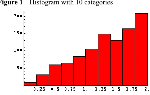
Figure 2 displays a histogram of an array, tbl, of 1000 random values from 0 to 2. (The table values only serve as data for graphing; each table entry is 2 times the
maximum of two random numbers.) The commands to generate the table and produce the histogram are as follows:
tbl = 2 * max(rand(1, 1000), rand(1, 1000)); hist(tbl)
MATLAB uses 10 intervals, so each interval length is 0.25 (see Figure 2).
Figure 1 Histogram with 10 categories
Quick Review Question 8
a. Generate a table, sinTbl, of 1000 values of the sine of a random floating point
number between 0 and π.
b. Display a histogram of sinTbl.
c. Display a histogram of sinTbl with 10 categories. d. Give the interval for the last category.
Maximum, Minimum, and Length
The MATLAB function max returns the maximum of a vector argument. Thus, the form of a call to the function can be as follows:
max([x1, x2, ... ])
In this case, the function returns the numerically largest of x1, x2, .... For example, the following invocation with four arguments returns the maximum argument, 7.
max([2, -4, 7, 3])
Another form of a call to the function, which follows, has a two-dimensional array of numbers as argument:
max([x11, x12,..., x1m; x21, x22,..., x2m; ...; xn1, xn2,..., xnm])
The result is a vector of the maximum in each column. The segment below generates a 3-by-3 array of numbers and returns the maximum values (3, 2, 5) in the columns:
lst = [-1, 2, -1; 0, 1, 5; 3, 2, 1];
max(lst)
To obtain the maximum (5) in the entire two-dimensional array, we take the maximum of this value, or the maximum of the maximum, as follows:
max(max(lst))
In a similar fashion, the MATLAB function min returns the minimum of a vector of numeric arguments; or in the case of a two-dimensional array, min returns a vector a minimum column values.
When we do not know the length of a vector, we can employ the length function, such as follows:
length(lst)
If lst were a matrix, this command would return its number of rows.
Quick Review Question 9 Start a new Script. In opening comments, have "MATLAB Tutorial 5 Answers" and your name. Save the file under the name
MATLABTutorial5Ans.m. In the file, preface this and all subsequent Quick Review Questions with a comment that has "%% QRQ" and the question number, such as follows:
%% QRQ 1 a
a. Write a segment to generate a list, lst, of 100 random floating point numbers between 0 and 1 and to display the maximum and minimum in the list.
Animation
One interesting use of a for loop is to draw several plots for an animation. In making the graphics, plots should have the same axis so that axes appear fixed during the animation. The segment below generates a sequence of plots of 0.5 sin(x), sin(x), 1.5 sin(x), ..., 5.0sin(x) with xvarying from 0 to 2π to illustrate the impact the coefficient has on
amplitude. However, for an effective demonstration, each graph must have the same display area, here from -5 to 5 on the y-axis.
x = 0:0.1:2*pi; for i = 1:10
y = 0.5 * i * sin(x); plot(x,y,'-');
axis([0 2*pi -5 5]);
end
However, the animation can be fairly slow and jerky as MATLAB generates the animation one frame at a time.
Alternatively, we can store the frames in a vector and later replay the sequence as a movie. Immediately after generating the i-th frame of the animation, we save the graph in a vector using getframe, as follows
M(i) = getframe;
After creating and storing all the frames, we show the animation with the movie
command, which has the vector, here M, and the number of times to show the movie as arguments. Thus, the following command displays the animation 10 times:
movie(M, 10)
To display the animation one time with 5 frames per second, include a third parameter, such as follows:
movie(M, 1, 5)
The adjusted sequence to generate and play a movie twice with 4 frames per second follows:
x = 0:0.1:2*pi; for i = 1:10
y = 0.5 * i * sin(x); plot(x,y,'-');
axis([0 2*pi -5, 5]);
M(i) = getframe;
end
Quick Review Question 10 The first two statements of following segment generate 10 random x- and y-coordinates between 0 and 1. We then plot the points as fairly large blue dots in a 1-by-1 rectangle. Adjust the code to generate 10 plots. The first graphics only displays the first point; the second graphics shows the first two points; and so forth. After execution, animate to show the points appearing one at a time. Why do we want to specify the plot range to be the same for each graphic?
xLst = rand(1, 10); yLst = rand(1, 10);
plot(xLst, yLst, 'ob', 'MarkerFaceColor', 'b') axis([0 1 0 1])
Quick Review Question 11 The function f below is the logistic function for constrained growth, where the initial population is 20, the carrying capacity is 1000, and the rate of change of the population is (1 + 0.2i) (see Module 2.3, "Constrained Growth"). We use the operators ./ and .* so that the function works with arrays of numbers, such as t = 0:0.1:3, as well as numbers. To see the effect of increasing the rate of change from (1 + 0.2(1)) = 1.2 to (1 + 0.2(10)) = 3.0, replace the assignment of 5 to i with the start of a for loop to generate 10 plots of f(t, i), where i varies from 1 to 10. Create a movie of the animation that plays five times.
clear('i', 'f', 't');
f = @(t, i) (1000*20)./((1000 - 20).*exp(-(1+0.2*i).*t) + 20); t = 0:0.1:3;
i = 5; % replace with for loop plot(t, f(t, i));