2
Chris Long & Naser Sayma
3
Heat Transfer
1
stedition
© 2009 Chris Long, Naser Sayma &
bookboon.com
4
Contents
1 Introduction 7
1.1 Heat Transfer Modes 7
1.2 System of Units 8
1.3 Conduction 8
1.4 Convection 12
1.5 Radiation 16
1.6 Summary 20
1.7 Multiple Choice assessment 21
2 Conduction 25
2.1 The General Conduction Equation 25
2.2 One-Dimensional Steady-State Conduction in Radial Geometries: 33
2.3 Fins and Extended Surfaces 38
2.4 Summary 47
2.5 Multiple Choice Assessment 48
Click on the ad to read more www.sylvania.com
We do not reinvent
the wheel we reinvent
light.
Fascinating lighting offers an infinite spectrum of possibilities: Innovative technologies and new markets provide both opportunities and challenges. An environment in which your expertise is in high demand. Enjoy the supportive working atmosphere within our global group and benefit from international career paths. Implement sustainable ideas in close cooperation with other specialists and contribute to influencing our future. Come and join us in reinventing light every day.
5
3 Convection 58
3.1 The convection equation 59
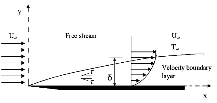
3.2 Flow equations and boundary layer 59
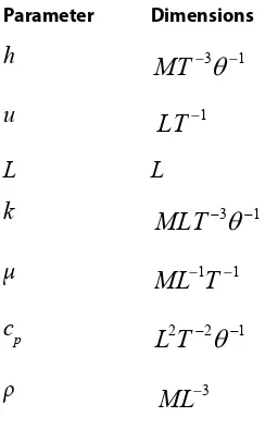
3.3 Dimensional analysis 71
3.4 Forced Convection relations 77
3.5 Natural convection 90
3.6 Summary 100
3.7 Multiple Choice Assessment 101
4 Radiation 108
4.1 Introduction 108
4.2 Radiative Properties 110
4.3 Kirchhoff ’s law of radiation 112
4.4 View factors and view factor algebra 112
4.4 Radiative Exchange Between a Number of Black Surfaces 115 4.5 Radiative Exchange Between a Number of Grey Surfaces 116
4.6 Radiation Exchange Between Two Grey Bodies 122
4.7 Summary 123
4.8 Multiple Choice Assessment 124
Click on the ad to read more Click on the ad to read more
EADS unites a leading aircraft manufacturer, the world’s largest helicopter supplier, a global leader in space programmes and a worldwide leader in global security solutions and systems to form Europe’s largest defence and aerospace group. More than 140,000 people work at Airbus, Astrium, Cassidian and Eurocopter,
in 90 locations globally, to deliver some of the industry’s most exciting projects.
An EADS internship offers the chance to use your theoretical knowledge and apply it first-hand to real situations and assignments during your studies. Given a high level of responsibility, plenty of
learning and development opportunities, and all the support you need, you will tackle interesting challenges on state-of-the-art products. We welcome more than 5,000 interns every year across disciplines ranging from engineering, IT, procurement and finance, to strategy, customer support, marketing and sales. Positions are available in France, Germany, Spain and the UK.
To find out more and apply, visit www.jobs.eads.com. You can also find out more on our EADS Careers Facebook page.
6
5 Heat Exchangers 129
5.1 Introduction 129
5.2 Classification of Heat Exchangers 130
5.3 The overall heat transfer coefficient 133
5.4 Analysis of Heat Exchangers 140
5.5 Summary 152
5.6 Multiple Choice Assessment 152
6 References 155
Click on the ad to read more Click on the ad to read more Click on the ad to read more
360°
thinking
.
© Deloitte & Touche LLP and affiliated entities.
7
1 Introduction
Energy is defined as the capacity of a substance to do work. It is a property of the substance and it can be transferred by interaction of a system and its surroundings. The student would have encountered these interactions during the study of Thermodynamics. However, Thermodynamics deals with the end states of the processes and provides no information on the physical mechanisms that caused the process to take place. Heat Transfer is an example of such a process. A convenient definition of heat transfer is energy in transition due to temperature differences. Heat transfer extends the Thermodynamic analysis by studying the fundamental processes and modes of heat transfer through the development of relations used to calculate its rate.
The aim of this chapter is to console existing understanding and to familiarise the student with the standard of notation and terminology used in this book. It will also introduce the necessary units.
1.1
Heat Transfer Modes
The different types of heat transfer are usually referred to as ‘modes of heat transfer’. There are three of these: conduction, convection and radiation.
• Conduction: This occurs at molecular level when a temperature gradient exists in a
medium, which can be solid or fluid. Heat is transferred along that temperature gradient by conduction.
• Convection: Happens in fluids in one of two mechanisms: random molecular motion which is termed diffusion or the bulk motion of a fluid carries energy from place to place. Convection can be either forced through for example pushing the flow along the surface or natural as that which happens due to buoyancy forces.
• Radiation: Occurs where heat energy is transferred by electromagnetic phenomenon, of which the sun is a particularly important source. It happens between surfaces at different temperatures even if there is no medium between them as long as they face each other.
8
1.2
System of Units
Before looking at the three distinct modes of transfer, it is appropriate to introduce some terms and units that apply to all of them. It is worth mentioning that we will be using the SI units throughout this book:
• The rate of heat flow will be denoted by the symbol Q. It is measured in Watts (W) and multiples such as (kW) and (MW).
• It is often convenient to specify the flow of energy as the heat flow per unit area which is also known as heat flux. This is denoted by q. Note that, q = Q/A where A is the area through which the heat flows, and that the units of heat flux are (W/m2).
• Naturally, temperatures play a major part in the study of heat transfer. The symbol T will be used for temperature. In SI units, temperature is measured in Kelvin or Celsius: (K) and (°C). Sometimes the symbol t is used for temperature, but this is not appropriate in the context of transient heat transfer, where it is convenient to use that symbol for time. Temperature difference is denoted in Kelvin (K).
The following three subsections describe the above mentioned three modes of heat flow in more detail. Further details of conduction, convection and radiation will be presented in Chapters 2, 3 and 4 respectively. Chapter 5 gives a brief overview of Heat Exchangers theory and application which draws on the work from the previous Chapters.
1.3 Conduction
9
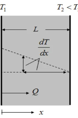
Figure 1.1 shows, in schematic form, a process of conductive heat transfer and identifies the key quantities to be considered:
Q: the heat flow by conduction in the x-direction (W)
A: the area through which the heat flows, normal to the x-direction (m2)
G[
G7
: the temperature gradient in the x-direction (K/m)These quantities are related by Fourier’s Law, a model proposed as early as 1822:
G[
G7
N
T
G[
G7
$
N
4
RU
(1.1)
A significant feature of this equation is the negative sign. This recognises that the natural direction for the flow of heat is from high temperature to low temperature, and hence down the temperature gradient.
The additional quantity that appears in this relationship is k, the thermal conductivity (W/m K) of the material through which the heat flows. This is a property of the particular heat-conducting substance and, like other properties, depends on the state of the material, which is usually specified by its temperature and pressure.
10
Considering the finite slab of material shown in Figure 1.1, we see that for one-dimensional conduction the temperature gradient is:
L - T T = d x
d T 2 1
2
Hence for this situation the transfer law can also be written
/ 7 7 N T /7 7 $ N
4 RU
(1.2)
=
C
k
r
a
(1.3)4Table 1.1 gives the values of thermal conductivity of some representative solid materials, for conditions of normal temperature and pressure. Also shown are values of another property characterising the flow of heat through materials, thermal diffusivity, which is related to the conductivity by:
Where ρ is the density in
NJ
P
of the material and C its specific heat capacity in Q-
NJ
.
.The thermal diffusivity indicates the ability of a material to transfer thermal energy relative to its ability to store it. The diffusivity plays an important role in unsteady conduction, which will be considered in Chapter 2.
As was noted above, the value of thermal conductivity varies significantly with temperature, even over the range of climatic conditions found around the world, let alone in the more extreme conditions of cold-storage plants, space flight and combustion. For solids, this is illustrated by the case of mineral wool, for which the thermal conductivity might change from 0.04 to 0.28 W/m K across the range 35 to -35 °C.
Material k W/m K α mm2/s Material k W/m K α mm2/s Copper Aluminium Mild steel Polyethylene Face Brick 350 236 50 0.5 1.0 115 85 13 0.15 0.75
Medium concrete block Dense plaster Stainless steel Nylon, Rubber Aerated concrete 0.5 0.5 14 0.25 0.15 0.35 0.40 4 0.10 0.40 Glass Fireclay brick Dense concrete Common brick 0.9 1.7 1.4 0.6 0.60 0.7 0.8 0.45 Wood, Plywood Wood-wool slab Mineral wool expanded Expanded polystyrene 0.15 0.10 0.04 0.035 0.2 0.2 1.2 1.0
11
For gases the thermal conductivities can vary significantly with both pressure and temperature. For liquids, the conductivity is more or less insensitive to pressure. Table 1.2 shows the thermal conductivities for typical gases and liquids at some given conditions.
Material k
[W/m K] Gases
Argon (at 300 K and 1 bar) Air (at 300 K and 1 bar) Air (at 400 K and 1 bar) Hydrogen (at 300 K and 1 bar) Freon 12 (at 300 K 1 bar)
0.018 0.026 0.034 0.180 0.070 Liquids
Engine oil (at 20oC) Engine oil (at 80oC) Water (at 20oC) Water (at 80oC) Mercury(at 27oC)
0.145 0.138 0.603 0.670 8.540
Table 1-2 Thermal conductivity for typical gases and liquids
Note the very wide range of conductivities encountered in the materials listed in Tables 1.1 and 1.2. Some part of the variability can be ascribed to the density of the materials, but this is not the whole story (Steel is more dense than aluminium, brick is more dense than water). Metals are excellent conductors of heat as well as electricity, as a consequence of the free electrons within their atomic lattices. Gases are poor conductors, although their conductivity rises with temperature (the molecules then move about more vigorously) and with pressure (there is then a higher density of energy-carrying molecules). Liquids, and notably water, have conductivities of intermediate magnitude, not very different from those for plastics. The low conductivity of many insulating materials can be attributed to the trapping of small pockets of a gas, often air, within a solid material which is itself a rather poor conductor.
Example 1.1
Calculate the heat conducted through a 0.2 m thick industrial furnace wall made of fireclay brick. Measurements made during steady-state operation showed that the wall temperatures inside and outside the furnace are 1500 and 1100 K respectively. The length of the wall is 1.2m and the height is 1m.
Solution
We first need to make an assumption that the heat conduction through the wall is one dimensional. Then we can use Equation 1.2:
L T T A k
12
The thermal conductivity for fireclay brick obtained from Table 1.1 is 1.7 W/m K
The area of the wall A = 1.2 × 1.0 = 1.2 m2
Thus:
W
4080
m
2
.
0
K
1100
K
1500
m
2
.
1
K
W/m
7
.
1
×
2×
−
=
=
Q
Comment: Note that the direction of heat flow is from the higher temperature inside to the lower temperature outside.
1.4 Convection
Convection heat transfer occurs both due to molecular motion and bulk fluid motion. Convective heat transfer may be categorised into two forms according to the nature of the flow: natural Convection and forced convection.
Click on the ad to read more Click on the ad to read more Click on the ad to read more Click on the ad to read more
We will turn your CV into
an opportunity of a lifetime
Do you like cars? Would you like to be a part of a successful brand? We will appreciate and reward both your enthusiasm and talent. Send us your CV. You will be surprised where it can take you.
13
In natural of ‘free’ convection, the fluid motion is driven by density differences associated with temperature changes generated by heating or cooling. In other words, fluid flow is induced by buoyancy forces. Thus the heat transfer itself generates the flow which conveys energy away from the point at which the transfer occurs.
In forced convection, the fluid motion is driven by some external influence. Examples are the flows of air induced by a fan, by the wind, or by the motion of a vehicle, and the flows of water within heating, cooling, supply and drainage systems. In all of these processes the moving fluid conveys energy, whether by design or inadvertently.
)ORRU
&HLOLQJ
5DGLDWRU
)UHHFRQYHFWLRQ
FHOO
6ROLGVXUIDFH
1DWXUDOFRQYHFWLRQ
)RUFHGFRQYHFWLRQ
Figure 1-2: Illustration of the process of convective heat transfer
The left of Figure 1.2 illustrates the process of natural convective heat transfer. Heat flows from the ‘radiator’ to the adjacent air, which then rises, being lighter than the general body of air in the room. This air is replaced by cooler, somewhat denser air drawn along the floor towards the radiator. The rising air flows along the ceiling, to which it can transfer heat, and then back to the lower part of the room to be recirculated through the buoyancy-driven ‘cell’ of natural convection.
The word ‘radiator’ has been written above in that way because the heat transfer from such devices is not predominantly through radiation; convection is important as well. In fact, in a typical central heating radiator approximately half the heat transfer is by (free) convection.
The right part of Figure 1.2 illustrates a process of forced convection. Air is forced by a fan carrying with it heat from the wall if the wall temperature is lower or giving heat to the wall if the wall temperature is lower than the air temperature.
If T1 is the temperature of the surface receiving or giving heat, and
T
∞ is the average temperature of the stream of fluid adjacent to the surface, then the convective heat transfer Q is governed by Newton’s law:RU
T
K
7
7
7
7
$
K
14
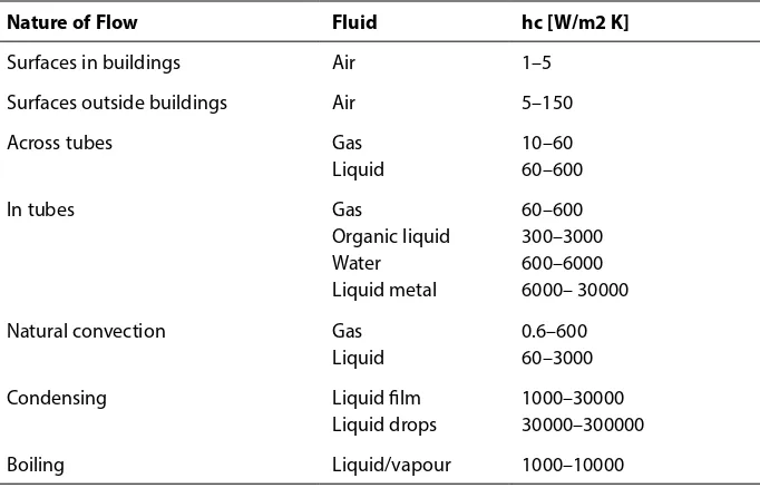
Another empirical quantity has been introduced to characterise the convective transfer mechanism. This is hc, the convective heat transfer coefficient, which has units [W/m2 K].
This quantity is also known as the convective conductance and as the film coefficient. The term film coefficient arises from a simple, but not entirely unrealistic, picture of the process of convective heat transfer at a surface. Heat is imagined to be conducted through a thin stagnant film of fluid at the surface, and then to be convected away by the moving fluid beyond. Since the fluid right against the wall must actually be at rest, this is a fairly reasonable model, and it explains why convective coefficients often depend quite strongly on the conductivity of the fluid.
Nature of Flow Fluid hc [W/m2 K]
Surfaces in buildings Air 1–5 Surfaces outside buildings Air 5–150 Across tubes Gas
Liquid
10–60 60–600 In tubes Gas
Organic liquid Water Liquid metal
60–600 300–3000 600–6000 6000– 30000 Natural convection Gas
Liquid
0.6–600 60–3000 Condensing Liquid film
Liquid drops
1000–30000 30000–300000 Boiling Liquid/vapour 1000–10000
Table 1-3 Representative range of convective heat transfer coefficient
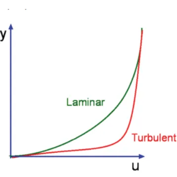
The film coefficient is not a property of the fluid, although it does depend on a number of fluid properties: thermal conductivity, density, specific heat and viscosity. This single quantity subsumes a variety of features of the flow, as well as characteristics of the convecting fluid. Obviously, the velocity of the flow past the wall is significant, as is the fundamental nature of the motion, that is to say, whether it is turbulent or laminar. Generally speaking, the convective coefficient increases as the velocity increases.
A great deal of work has been done in measuring and predicting convective heat transfer coefficients. Nevertheless, for all but the simplest situations we must rely upon empirical data, although numerical methods based on computational fluid dynamics (CFD) are becoming increasingly used to compute the heat transfer coefficient for complex situations.
15
Example 1.2
A refrigerator stands in a room where the air temperature is 20oC. The surface temperature on the outside
of the refrigerator is 16oC. The sides are 30 mm thick and have an equivalent thermal conductivity of
0.1 W/m K. The heat transfer coefficient on the outside 9 is 10 W/m2K. Assuming one dimensional conduction through the sides, calculate the net heat flow and the surface temperature on the inside.
Solution
Let
T
s,i andT
s,obe the inside surface and outside surface temperatures, respectively andT
f the fluid temperature outside.The rate of heat convection per unit area can be calculated from Equation 1.3:
)
(
T
s,oT
fh
q
=
−
:P
u
T
Click on the ad to read more Click on the ad to read more Click on the ad to read more Click on the ad to read more Click on the ad to read more
Linköping University –
innovative, highly ranked,
European
Interested in Engineering and its various branches? Kick-start your career with an English-taught master’s degree.
16
This must equal the heat conducted through the sides. Thus we can use Equation 1.2 to calculate the surface temperature:
L
T
T
k
q
=
−
s,o−
s,iu
7
VLC
T
s,i=
4
°
Comment: This example demonstrates the combination of conduction and convection heat transfer relations to establish the desired quantities.
1.5 Radiation
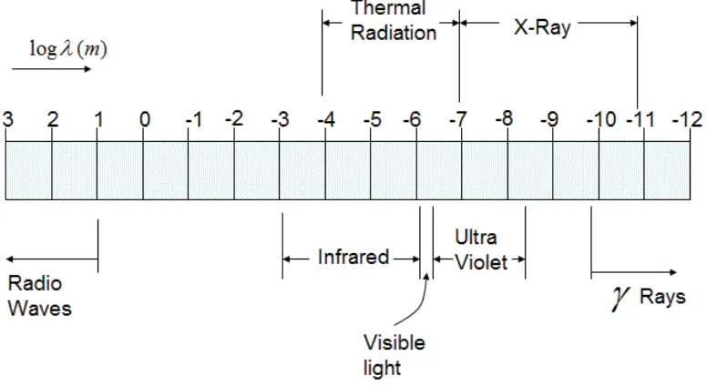
While both conductive and convective transfers involve the flow of energy through a solid or fluid substance, no medium is required to achieve radiative heat transfer. Indeed, electromagnetic radiation travels most efficiently through a vacuum, though it is able to pass quite effectively through many gases, liquids and through some solids, in particular, relatively thin layers of glass and transparent plastics.
Figure 1-3: Illustration of electromagnetic spectrum
Figure 1.3 indicates the names applied to particular sections of the electromagnetic spectrum where the band of thermal radiation is also shown. This includes:
• the rather narrow band of visible light;
17
Our immediate interest is thermal radiation. It is of the same family as visible light and behaves in the same general fashion, being reflected, refracted and absorbed. These phenomena are of particular importance in the calculation of solar gains, the heat inputs to buildings from the sun and radiative heat transfer within combustion chambers.
It is vital to realise that every body, unless at the absolute zero of temperature, both emits and absorbs energy by radiation. In many circumstances the inwards and outwards transfers nearly cancel out, because the body is at about the same temperature as its surroundings. This is your situation as you sit reading these words, continually exchanging energy with the surfaces surrounding you.
In 1884 Boltzmann put forward an expression for the net transfer from an idealised body (Black body) with surface area A1 at absolute temperature T1 to surroundings at uniform absolute temperature T2:
RU
7
7
T
7
7
$
4
V
V
(1.4)with
σ
the Stefan-Boltzmann constant, which has the value 5.67 × 10⁻⁸ W/m2 K4 and T [K] = T [°C] + 273 is the absolute temperature.The bodies considered above are idealised, in that they perfectly absorb and emit radiation of all wave-lengths. The situation is also idealised in that each of the bodies that exchange radiation has a uniform surface temperature. A development of Boltzmann’s law which allows for deviations from this pattern is
7 7 $ )
4
V
H
(1.5)With ε the emissivity, or emittance, of the surface A1, a dimensionless factor in therange 0 to 1,
F12 is the view factor, or angle factor, giving the fraction of the radiation from A1 that falls on the area A2 at temperature T2, and therefore also in the range 0 to 1.
Another property of the surface is implicit in this relationship: its absorbtivity. This has been taken to be equal to the emissivity. This is not always realistic. For example, a surface receiving short-wave-length radiation from the sun may reject some of that energy by re-radiation in a lower band of wave-lengths, for which the emissivity is different from the absorbtivity for the wave-lengths received.
18
The values quoted in the table are averages over a range of radiation wave-lengths. For most materials, considerable variations occur across the spectrum. Indeed, the surfaces used in solar collectors are chosen because they possess this characteristic to a marked degree. The emissivity depends also on temperature, with the consequence that the radiative heat transfer is not exactly proportional to T3.
An ideal emitter and absorber is referred to as a ‘black body’, while a surface with an emissivity less than unity is referred to as ‘grey’. These are somewhat misleading terms, for our interest here is in the infra-red spectrum rather than the visible part. The appearance of a surface to the eye may not tell us much about its heat-absorbing characteristics.
Ideal ‘black’ body White paint Gloss paint Brick Rusted steel
1.00 0.97 0.9 0.9 0.8
Aluminium paint Galvanised steel Stainless steel Aluminium foil Polished copper Perfect mirror
0.5 0.3 0.15 0.12 0.03 0
Table 1-4 Representative values of emissivity
Click on the ad to read more Click on the ad to read more Click on the ad to read more Click on the ad to read more Click on the ad to read more Click on the ad to read more
as a
e
s
al na
or o
eal responsibili�
I joined MITAS because
Maersk.com/Mitas�e Graduate Programme for Engineers and Geoscientists
as a
e
s
al na
or o
Month 16
I was a construction
supervisor in
the North Sea
advising and
helping foremen
solve problems
I was a
he
s
Real work International opportunities �ree work placements
al Internationa
or �ree wo
al na
or o
I wanted
real responsibili�
I joined MITAS because
19
Although it depends upon a difference in temperature, Boltzmann’s Law (Equations 1.4, 1.5) does not have the precise form of the laws for conductive and convective transfers. Nevertheless, we can make the radiation law look like the others. We introduce a radiative heat transfer coefficient or radiative conductance through
4
K
U$
7
7
(1.6)
Comparison with the developed form of the Boltzmann Equation (1.5), plus a little algebra, gives
)
T
+
T
(
)
T
+
T
(
F
=
)
T
-T
(
A
Q
=
h
12 1 2 12 222 1 1
r
e
σ
9
If the temperatures of the energy-exchanging bodies are not too different, this can be approximated by
7 )
K
DY
U
H
V
(1.7)where Tav is the average of the two temperatures.
Obviously, this simplification is not applicable to the case of solar radiation. However, the temperatures of the walls, floor and ceiling of a room generally differ by only a few degrees. Hence the approximation given by Equation (1.7) is adequate when transfers between them are to be calculated.
Example 1.3
Surface A in the Figure is coated with white paint and is maintained at temperature of 200oC. It is located
directly opposite to surface B which can be considered a black body and is maintained ate temperature of 800oC. Calculate the amount of heat that needs to be removed from surface A per unit area to maintain
its constant temperature.
Solution
20
The heat gained by surface A by radiation from surface B can be computed from Equation 1.5:
$
R& %R&
$ %
$%
7
7
)
T
H
V
The emissivity of white coated paint is 0.97 from Table 1.4
Thus
:P
u
u
u
T
This amount of heat needs to be removed from surface A by other means such as conduction, convection or radiation to other surfaces to maintain its constant temperature.
1.6 Summary
This chapter introduced some of the basic concepts of heat transfer and indicates their significance in the context of engineering applications.
We have seen that heat transfer can occur by one of three modes, conduction, convection and radiation. These often act together. We have also described the heat transfer in the three forms using basic laws as follows:
@
:
>
G[
G7
N$
4
Conduction:
Where thermal conductivity k [W/m K] is a property of the material
21
Where the convective coefficient h [W/m2 K] depends on the fluid properties and motion.
Radiation heat exchange between two surfaces of temperatures T1 and T2:
7 7 $ )
4
V
H
Where ε is the Emissivity of surface 1 and F12 is the view factor.
Typical values of the relevant material properties and heat transfer coefficients have been indicated for common materials used in engineering applications.
1.7
Multiple Choice assessment
1. The units of heat flux are:
• Watts
• Joules
• Joules / meters2
• Watts / meters2
• Joules / Kg K
Click on the ad to read more Click on the ad to read more Click on the ad to read more Click on the ad to read more Click on the ad to read more Click on the ad to read more Click on the ad to read more Sweden
www.teknat.umu.se/english
Think Umeå. Get a Master’s degree!
• modern campus • world class research • 31 000 students
• top class teachers • ranked nr 1 by international students
Master’s programmes:
22 2. The units of thermal conductivity are:
• Watts / meters2 K
• Joules
• Joules / meters2
• Joules / second meter K
• Joules / Kg K
3. The heat transfer coefficient is defined by the relationship
• h = m Cp ΔT
• h = k / L
• h = q / ΔT
• h = Nu k / L
• h = Q / ΔT
4. Which of these materials has the highest thermal conductivity?
• air
• water
• mild steel
• titanium
• aluminium
5. Which of these materials has the lowest thermal conductivity?
• air
• water
• mild steel
• titanium
• aluminium
6. In which of these is free convection the dominant mechanism of heat transfer?
• heat transfer to a piston head in a diesel engine combustion chamber
• heat transfer from the inside of a fan-cooled p.c.
• heat transfer to a solar heating panel
• heat transfer on the inside of a central heating panel radiator
23 7. Which of these statements is not true?
• conduction can occur in liquids
• conduction only occurs in solids
• thermal radiation can travel through empty space
• convection cannot occur in solids
• gases do not absorb thermal radiation
8. What is the heat flow through a brick wall of area 10m2, thickness 0.2m, k = 0.1 W/m K with a surface temperature on one side of 20ºC and 10ºC on the other?
• 50 Watts
• 50 Joules
• 50 Watts / m2
• 200 Watts
• 200 Watts / m2
9. The governing equations of fluid motion are known as:
• Maxwell’s equations
• C.F.D.
• Reynolds – Stress equations
• Lame’s equations
• Navier – Stokes equations
10. A pipe of surface area 2m2 has a surface temperature of 100ºC, the adjacent fluid is at 20ºC, the heat transfer coefficient acting between the two is 20 W/m2K. What is the heat flow by convection?
• 1600 W
• 3200 W
• 20 W
• 40 W
• zero
11. The value of the Stefan-Boltzmann constant is:
• 56.7 × 10⁻⁶ W/m2K4
• 56.7 × 10⁻⁹ W/m2K4
• 56.7 × 10⁻⁶ W/m2K
• 56.7 × 10⁻⁹ W/m2K
24
12. Which of the following statements is true: Heat transfer by radiation….
• only occurs in outer space
• is negligible in free convection
• is a fluid phenomenon and travels at the speed of the fluid
• is an acoustic phenomenon and travels at the speed of sound
• is an electromagnetic phenomenon and travels at the speed of light
13. Calculate the net thermal radiation heat transfer between two surfaces. Surface A, has a temperature of 100ºC and Surface B, 200ºC. Assume they are sufficiently close so that all the radiation leaving A is intercepted by B and vice-versa. Assume also black-body behaviour.
• 85 W
• 85 W / m2
• 1740 W
• 1740 W / m2
• none of these
14. The different modes of heat transfer are:
• forced convection, free convection and mixed convection
• conduction, radiation and convection
• laminar and turbulent
• evaporation, condensation and boiling
• cryogenic, ambient and high temperature
15. Mixed convection refers to:
• combined convection and radiation
• combined convection and conduction
• combined laminar and turbulent flow
• combined forced and free convection
• combined forced convection and conduction
16. The thermal diffusivity, a, is defined as:
• = m Cp / k
• = k Cp / r
• = k / r Cp
• = h L / k
25
2 Conduction
2.1
The General Conduction Equation
Conduction occurs in a stationary medium which is most likely to be a solid, but conduction can also occur in fluids. Heat is transferred by conduction due to motion of free electrons in metals or atoms in non-metals. Conduction is quantified by Fourier’s law: the heat flux, q, is proportional to the temperature gradient in the direction of the outward normal. e.g. in the x-direction:
G[
G7
T
[v
(2.1):
P
G[
G7
N
T
[ (2.2)The constant of proportionality, k is the thermal conductivity and over an area A, the rate of
heat flow in the x-direction, Qx is
:
G[
G7
$
N
4
[(2.3)
26
Conduction may be treated as either steady state, where the temperature at a point is constant with time, or as time dependent (or transient) where temperature varies with time.
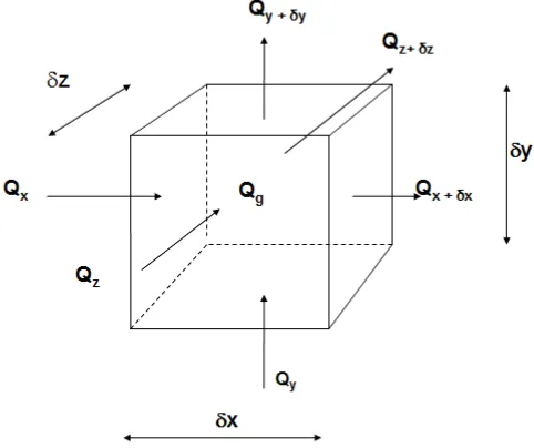
The general, time dependent and multi-dimensional, governing equation for conduction can be derived from an energy balance on an element of dimensions δx, δy, δz.
Consider the element shown in Figure 2.1. The statement of energy conservation applied to this element in a time period δt is that:
heat flow in + internal heat generation = heat flow out + rate of increase in internal energy
t
T
C
m
Q
Q
Q
Q
Q
Q
Q
x y z g x x y y z z∂
∂
+
+
+
=
+
+
+
+d +d +d (2.4)or
0
=
∂
∂
+
+
−
+
−
+
−
+ + +t
T
C
m
Q
Q
Q
Q
Q
Q
Q
x x dx y y dy z z dz g (2.5)As noted above, the heat flow is related to temperature gradient through Fourier’s Law, so:
Figure 2-1 Heat Balance for conduction in an infinitismal element
G[
G7
]
\
N
G[
G7
$
N
4
[G
G
G\
G7
]
[
N
G\
G7
$
N
4
\G
G
(2.6)G[
G7
\
[
N
G]
G7
$
N
27 Using a Taylor series expansion:
+
∂
∂
+
∂
∂
+
∂
∂
+
=
+ 3 3
3 2 2 2
!
3
1
!
2
1
x
x
Q
x
x
Q
x
x
Q
Q
Q
x x xx x
x d
d
d
d
(2.7)For small values of δx it is a good approximation to ignore terms containing δx2 and higher order terms, So:
∂
∂
−
∂
∂
=
∂
∂
≅
−
+x
T
k
x
z
y
x
x
x
Q
Q
Q
x x xx d
d
d
d
d
(2.8)A similar treatment can be applied to the other terms. For time dependent conduction in three dimensions (x,y,z), with internal heat generation qg(W/m3)=Qg/dxdydz:
t
T
C
q
z
T
k
z
y
T
k
y
x
T
k
x
g∂
∂
=
+
∂
∂
−
∂
∂
+
∂
∂
−
∂
∂
+
∂
∂
−
∂
∂
r
(2.9)For constant thermal conductivity and no internal heat generation (Fourier’s Equation):
t
T
k
C
z
T
y
T
x
T
∂
∂
=
∂
∂
+
∂
∂
+
∂
∂
r
2 2 2 2 2 2 (2.10)Where (k/rC) is known as α, the thermal diffusivity (m2/s).
For steady state conduction with constant thermal conductivity and no internal heat generation
0
2 2 2 2 2 2=
∂
∂
+
∂
∂
+
∂
∂
z
T
y
T
x
T
(2.11)Similar governing equations exist for other co-ordinate systems. For example, for 2D cylindrical coordinate system (r, z). In this system there is an extra term involving 1/r which accounts for the variation in area with r.
0
1
2 2 2 2=
∂
∂
+
∂
∂
+
∂
∂
r
T
r
r
T
z
T
(2.12)For one-dimensional steady state conduction (in say the x-direction)
G[
7
G
(2.13)28
A meaningful solution to one of the above conduction equations is not possible without information about what happens at the boundaries (which usually coincide with a solid-fluid or solid-solid interface). This information is known as the boundary conditions and in conduction work there are three main types:
1. where temperature is specified, for example the temperature of the surface of a turbine disc, this is known as a boundary condition of the 1st kind;
2. where the heat flux is specified, for example the heat flux from a power transistor to its heat sink, this is known as a boundary condition of the 2nd kind;
3. where the heat transfer coefficient is specified, for example the heat transfer coefficient acting on a heat exchanger fin, this is known as a boundary condition of the 3rd kind.
2.1.1 Dimensionless Groups for Conduction
There are two principal dimensionless groups used in conduction. These are: The Biot number, %L K/N and The Fourier number, )R DW/.
It is customary to take the characteristic length scale L as the ratio of the volume to exposed surface area of the solid.
29
The Biot number can be thought of as the ratio of the thermal resistance due to conduction (L/k) to the thermal resistance due to convection 1/h. So for Bi << 1, temperature gradients within the solid are negligible and for Bi > 1 they are not. The Fourier number can be thought of as a time constant for conduction. For )R, time dependent effects are significant and for )R!! they are not.
2.1.2 One-Dimensional Steady State Conduction in Plane Walls
In general, conduction is multi-dimensional. However, we can usually simplify the problem to two or even one-dimensional conduction. For one-dimensional steady state conduction (in say the x-direction):
G[
7
G
(2.14)From integrating twice:
2
1
x
C
C
T
=
+
where the constants C1 and C2 are determined from the boundary conditions. For example if the temperature is specified (1st Kind) on one boundary T = T1 at x = 0 and there is convection into a surrounding fluid (3rd Kind) at the other boundary
N
G7
G[
K
7
7
IOXLG at x = L then:¿
¾
½
¯
®
7
7
IOXLGN
K[
7
7
(2.15)which is an equation for a straight line.
To analyse 1-D conduction problems for a plane wall write down equations for the heat flux q. For example, the heat flows through a boiler wall with convection on the outside and convection on the inside:
)
(
T
T
1h
q
=
inside inside−
N / 7 7
T
)
(
2 outside outsideT
T
h
q
=
−
Rearrange, and add to eliminate T1 and T2 (wall temperatures)
+
+
−
=
outside inside
otside inside
h
k
h
T
T
q
1
1
30
Note the similarity between the above equation with I = V / R (heat flux is the analogue of electrical current, temperature is of voltage and the denominator is the overall thermal resistance, comprising individual resistance terms from convection and conduction.
In building services it is common to quote a ‘U’ value for double glazing and building heat loss calculations. This is called the overall heat transfer coefficient and is the inverse of the overall thermal resistance.
+
+
=
outsideinside
k
h
h
U
1
1
1
1
(2.17)2.1.3 The Composite Plane Wall
The extension of the above to a composite wall (Region 1 of width L1, thermal conductivity k1, Region 2 of width L2 and thermal conductivity k2 . . . . etc. is fairly straightforward.
+
+
+
+
−
=
outside inside otside insideh
k
L
k
L
k
L
h
T
T
q
1
1
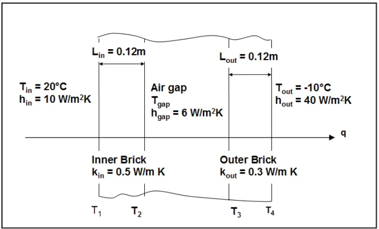
3 3 2 2 1 1 (2.18) Example 2.1The walls of the houses in a new estate are to be constructed using a ‘cavity wall’ design. This comprises an inner layer of brick (k = 0.5 W/m K and 120 mm thick), an air gap and an outer layer of brick (k = 0.3 W/m K and 120 mm thick). At the design condition the inside room temperature is 20ºC, the outside air temperature is -10ºC; the heat transfer coefficient on the inside is 10 W/m2 K, that on the outside 40 W/m2 K, and that in the air gap 6 W/m2 K. What is the heat flux through the wall?
31
Note the arrow showing the heat flux which is constant through the wall. This is a useful concept, because we can simply write down the equations for this heat flux.
Convection from inside air to the surface of the inner layer of brick
)
(
T
T
1h
q
=
in in−
Conduction through the inner layer of brick
)
(
/
L
T
1T
2k
q
=
in in−
Convection from the surface of the inner layer of brick to the air gap
)
(
2 gapgap
T
T
h
q
=
−
Convection from air gap to the surface of the outer layer of brick
)
(
T
T
3h
q
=
gap gap−
Click on the ad to read more Click on the ad to read more Click on the ad to read more Click on the ad to read more Click on the ad to read more Click on the ad to read more Click on the ad to read more Click on the ad to read more Click on the ad to read more Click on the ad to read more
Open your mind to
new opportunities
With 31,000 students, Linnaeus University is one of the larger universities in Sweden. We are a modern university, known for our strong international profile. Every year more than 1,600 international students from all over the world choose to enjoy the friendly atmosphere and active student life at Linnaeus University. Welcome to join us!
Bachelor programmes in
Business & Economics | Computer Science/IT | Design | Mathematics
Master programmes in
Business & Economics | Behavioural Sciences | Computer Science/IT | Cultural Studies & Social Sciences | Design | Mathematics | Natural Sciences | Technology & Engineering
32 Conduction through the outer layer of brick
)
(
/
L
T
3T
4k
q
=
out out−
Convection from the surface of the outer layer of brick to the outside air
)
(
4 outout
T
T
h
q
=
−
The above provides six equations with six unknowns (the five temperatures T1, T2, T3, T4 and
T
gap and the heat flux q). They can be solved simply by rearranging with the temperatures on the left hand side.in
in
T
q
h
T
)
/
(
−
1=
(
k
inL
in)
q
T
T
)
/
/
(
2−
1=
gap
gap
q
h
T
T
)
/
(
2−
=
gap
gap
T
q
h
T
)
/
(
−
3=
(
k
outL
out)
q
T
T
)
/
/
(
3−
4=
out
out
q
h
T
T
)
/
(
4−
=
Then by adding, the unknown temperatures are eliminated and the heat flux can be found directly
33
It is instructive to write out the separate terms in the denominator as it can be seen that the greatest thermal resistance is provided by the outer layer of brick and the least thermal resistance by convection on the outside surface of the wall. Once the heat flux is known it is a simple matter to use this to find each of the surface temperatures. For example,
(
q
h
out)
T
outT
4=
/
+
7
& 7 q
Thermal Contact Resistance
In practice when two solid surfaces meet then there is not perfect thermal contact between them. This can be accounted for using an appropriate value of thermal contact resistance – which can be obtained either from experimental results or published, tabulated data.
2.2
One-Dimensional Steady-State Conduction in Radial Geometries:
Pipes, pressure vessels and annular fins are engineering examples of radial systems. The governing equation for steady-state one-dimensional conduction in a radial system is
GU
G7
U
GU
7
G
(2.19)From integrating twice:
2 1ln(x) C
C
T = + , and the constants are determined from the boundary conditions, e.g. if T = T1 at r = r1 and T = T2 at r = r2, then:
=
−
−
)
/
ln(
)
/
ln(
1 2
1
1 2
1
r
r
r
r
T
T
T
T
(2.20)
Similarly since the heat flow 4 N$G7GU, then for a length L (in the axial or ‘z’ direction) the heat flow can be found from differentiating Equation 2.20.
(
)
)
/
ln(
2
1 2
1 2
r
r
T
T
K
L
34 To analyse 1-D radial conduction problems:
Write down equations for the heat flow Q (not the flux, q, as in plane systems, since in a radial system the area is not constant, so q is not constant). For example, the heat flow through a pipe wall with convection on the outside and convection on the inside:
)
(
2
r
1L
h
T
T
1Q
=
π
inside inside−
)
/
ln(
/
)
(
2
L
k
T
1T
2r
2r
1Q
=
π
−
)
(
2
r
2L
h
outsideT
2T
outsiedQ
=
π
−
Rearrange, and add to eliminate T1 and T2 (wall temperatures)
+
+
−
=
outside inside
outside inside
h
r
k
r
r
h
r
T
T
L
Q
2 1
2
1
1
)
/
ln(
1
)
(
2
π
(2.22)
The extension to a composite pipe wall (Region 1 of thermal conductivity k1, Region 2 of thermal conductivity k2 . . . . etc.) is fairly straightforward.
Click on the ad to read more Click on the ad to read more Click on the ad to read more Click on the ad to read more Click on the ad to read more Click on the ad to read more Click on the ad to read more Click on the ad to read more Click on the ad to read more Click on the ad to read more Click on the ad to read more
81,000 km
In the past four years we have drilled
That’s more than twice around the world.
What will you be? Who are we?
We are the world’s leading oilfield services company. Working globally—often in remote and challenging locations—we invent, design, engineer, manufacture, apply, and maintain technology to help customers find and produce oil and gas safely.
Who are we looking for?
We offer countless opportunities in the following domains:
n Engineering, Research, and Operations nGeoscience and Petrotechnical
nCommercial and Business
If you are a self-motivated graduate looking for a dynamic career, apply to join our team.
35
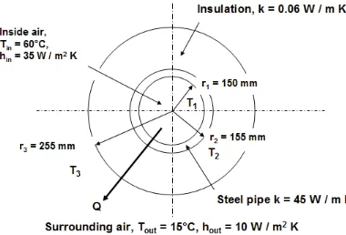
Example 2.2
The Figure below shows a cross section through an insulated heating pipe which is made from steel (k = 45 W / m K) with an inner radius of 150 mm and an outer radius of 155 mm. The pipe is coated with 100 mm thickness of insulation having a thermal conductivity of k = 0.06 W / m K. Air at Ti = 60°C flows through the pipe and the convective heat transfer coefficient from the air to the inside of the pipe has a value of hi = 35 W / m2 K. The outside surface of the pipe is surrounded by air which is at 15°C and the convective heat transfer coefficient on this surface has a value of ho = 10 W / m2 K. Calculate the heat loss through 50 m of this pipe.
Solution
Figure 2-3: Conduction through a radial wall
Unlike the plane wall, the heat flux is not constant (because the area varies with radius). So we write down separate equations for the heat flow, Q.
Convection from inside air to inside of steel pipe
)
(
2
r
1L
h
T
T
1Q
=
π
in in−
Conduction through steel pipe
)
/
ln(
/
)
(
2
L
k
T
1T
2r
2r
136 Conduction through the insulation
)
/
ln(
/
)
(
2
L
k
T
2T
3r
3r
2Q
=
π
insulation−
Convection from outside surface of insulation to the surrounding air
)
(
2
r
3L
h
outT
3T
outQ
=
π
−
Following the practice established for the plane wall, rewrite in terms of temperatures on the left hand side and then add to eliminate the unknown values of temperature, giving
+
+
+
−
=
out insulation steel in o ih
r
k
r
r
k
r
r
h
r
T
T
L
Q
3 2 3 1 2 11
)
/
ln(
)
/
ln(
1
)
(
2
π
(2.23)¸
¹
·
¨
©
§
u
¸
¹
·
¨
©
§
¸
¹
·
¨
©
§
¸
¹
·
¨
©
§
u
u
u
OQ
OQ
S
4
Watts
Q
=
1592
Again, the thermal resistance of the insulation is seen to be greater than either the steel or the two resistances due to convection.
Critical Insulation Radius
Adding more insulation to a pipe does not always guarantee a reduction in the heat loss. Adding more insulation also increases the surface area from which heat escapes. If the area increases more than the thermal resistance then the heat loss is increased rather than decreased.
The so-called critical insulation radius is the largest radius at which adding more insulation will create an increase in the heat loss
ext ins
crit
k
k
37
Example 2.3
Find the critical insulation radius for the previous question.
Solution:
ext ins
crit
k
h
r
=
/
FULWU
PP
U
FULWSo for r3 > 6 mm, adding more insulation, as intended, will reduce the heat loss.
Click on the ad to read more Click on the ad to read more Click on the ad to read more Click on the ad to read more Click on the ad to read more Click on the ad to read more Click on the ad to read more Click on the ad to read more Click on the ad to read more Click on the ad to read more Click on the ad to read more Click on the ad to read more
“The perfect start
of a successful,
international career.”
CLICK HERE
to discover why both socially and academically the University
of Groningen is one of the best places for a student to be
www.rug.nl/feb/education
38
2.3
Fins and Extended Surfaces
Figure 2-4: Examples of fins (a) motorcycel engine, (b) heat sink
Fins and extended surfaces are used to increase the surface area and therefore enhance the surface heat transfer. Examples are seen on: motorcycle engines, electric motor casings, gearbox casings, electronic heat sinks, transformer casings and fluid heat exchangers. Extended surfaces may also be an unintentional product of design. Look for example at a typical block of holiday apartments in a ski resort, each with a concrete balcony protruding from external the wall. This acts as a fin and draws heat from the inside of each apartment to the outside. The fin model may also be used as a first approximation to analyse heat transfer by conduction from say compressor and turbine blades.
2.3.1 General Fin Equation
The general equation for steady-state heat transfer from an extended surface is derived by considering the heat flows through an elemental cross-section of length δx, surface area δAs and cross-sectional area Ac. Convection occurs at the surface into a fluid where the heat transfer coefficient is h and the temperature Tfluid.
39
Writing down a heat balance in words: heat flow into the element = heat flow out of the element + heat transfer to the surroundings by convection. And in terms of the symbols in Figure 2.5
)
(
fluids x
x
x
Q
h
A
T
T
Q
=
+d+
d
−
(2.24)From Fourier’s Law.
G[
G7
$
N
4
[ F (2.25)and from a Taylor’s series, using Equation 2.25
[
G[
G7
$
N
G[
G
4
4
[ G[ [ F¸
G
¹
·
¨
©
§
(2.26)and so combining Equations 2.24 and 2.26
¸
¹
·
¨
©
§
IOXLG VF
G7
G[
[
K
$
7
7
$
N
G[
G
G
G
(2.27)
The term on the left is identical to the result for a plane wall. The difference here is that the area is not constant with x. So, using the product rule to multiply out the first term on the left hand-side, gives:
V IOXLG F F F7
7
G[
G$
N
$
K
G[
G7
G[
G$
$
G[
7
G
(2.28)The simplest geometry to consider is a plane fin where the cross-sectional area, Ac and surface area As are both uniform. Putting
Θ
=
T
−
T
fluid and lettingm
2=
h
p
/
A
ck
, where P is the perimeter of the cross-section4
4
P
G[
G
(2.29)The general solution to this is Θ = C1emx + C2e-mx, where the constants C1 and C2, depend on the boundary conditions.
It is useful to look at the following four different physical configurations:
N.B. sinh, cosh and tanh are the so-called hyperbolic sine, cosine and tangent functions defined by:
FRVK
VLQK
WDQK
DQG
VLQK
FRVK
[
[
[
H
H
[
H
H
40 Convection from the fin tip (
h
x=L=
h
tip)
`
VLQK
^
FRVK
`
VLQK
^
FRVK
P/
N
P
K
P/
[
/
P
N
P
K
[
/
P
7
7
7
7
WLS WLS IOXLG EDVH IOXLG (2.31)where
h
base=
h
x=0.`
VLQK
^
FRVK
`
FRVK
^
VLQK
P/
N
P
K
P/
P/
N
P
K
P/
7
7
$
N
3
K
4
WLS WLS IOXLG EDVH F(2.32)
Adiabatic Tip (htip = 0 in Equation 2.32)
4
4
P
G[
G
(2.33) WDQKK3N$ 7 7 P/
4 F EDVH IOXLG (2.34)
Click on the ad to read more Click on the ad to read more Click on the ad to read more Click on the ad to read more Click on the ad to read more Click on the ad to read more Click on the ad to read more Click on the ad to read more Click on the ad to read more Click on the ad to read more Click on the ad to read more Click on the ad to read more Click on the ad to read more
41 3. Tip at a specified temperature (Tx = L)
VLQK VLQK VLQK P/ [ / P P[ 7 7 7 7 7 7 7
7 EDVH IOXLG
IOXLG / [ IOXLG EDVH IOXLG °¿ ° ¾ ½ °¯ ° ® ¸ ¸ ¹ · ¨ ¨ © § (2.35)
VLQK
FRVK
P/
7
7
7
7
P/
7
7
$
N
3
K
4
EDVH IOXLGIOXLG / [ IOXLG EDVH F
°¿
°
¾
½
°¯
°
®
¸
¸
¹
·
¨
¨
©
§
(2.36)Infinite Fin
(
T
=
T
fluida
t
x
=
∞
)
P[ IOXLG EDVH IOXLG
H
7
7
7
7
(2.37))
(
)
(
h
P
k
A
c 1/2T
baseT
fluidQ
=
−
(2.38)2.3.2 Fin Performance
The performance of a fin is characterised by the fin effectiveness and the fin efficiency
Fin effectiveness,
e
fin=
fin
e
fin heat transfer rate / heat transfer rate that would occur in the absence of the fin F EDVH IOXLGILQ
4
K$
7
7
H
(2.39)which for an infinite fin becomes, Q given by
F
ILQ 3N K$
H
(2.40)Fin efficiency,
η
fin=
fin
η
actual heat transfer through the fin / heat transfer that would occur if the entire fin were at the base temperature. V EDVH IOXLGILQ
4
K$
7
7
K
(2.41)
which for an infinite fin becomes, with Q given by Equation 2.38
F V
ILQ 3N$ K$
42
Example 2.3
The design of a single ‘pin fin’ which is to be used in an array of identical pin fins on an electronics heat sink is shown in Figure 2.6. The fin is made from cast aluminium, k = 180 W / m K, the diameter is 3 mm and the length 15 mm. There is a heat transfer coefficient of 30 W / m2 K between the surface of the fin and surrounding air which is at 25°C.
1. Use the expression for a fin with an adiabatic tip to calculate the heat flow through a single pin fin when the base has a temperature of 55°C.
2. Calculate also the efficiency and the effectiveness of this fin design. 3. How long would this fin have to be to be considered “infinite”?
Figure 2-6 Pin Fin design
Solution
For a fin with an adiabatic tip
WDQK
K3N$ 7 7 P/
4 F EDVH IOXLG
For the above geometry
P
G
3
S
u
P
G
$
FS
u
K3
N
$
/
u
u
u
u
u
/
P
FWDQK
P/
u
u
u
u
u
u
u
4
:DWWV
43 Fin efficiency
V EDVH IOXLGILQ
4
K$
7
7
K
P
G
$
FS
u
u u u
ILQ
K
ILQK
Fin effectiveness F EDVH IOXLGILQ
4
K$
7
7
H
u u ILQH
ILQH
Click on the ad to read more Click on the ad to read more Click on the ad to read more Click on the ad to read more Click on the ad to read more Click on the ad to read more Click on the ad to read more Click on the ad to read more Click on the ad to read more Click on the ad to