Machine Learning
for Dynamic
Software Analysis
Potentials and Limits
Sta
te
-of-the
-Ar
t
Sur
vey
LNCS 11026
123
International Dagstuhl Seminar 16172
Dagstuhl Castle, Germany, April 24–27, 2016
Revised Papers
Commenced Publication in 1973 Founding and Former Series Editors:
Gerhard Goos, Juris Hartmanis, and Jan van Leeuwen
Editorial Board
David HutchisonLancaster University, Lancaster, UK Takeo Kanade
Carnegie Mellon University, Pittsburgh, PA, USA Josef Kittler
University of Surrey, Guildford, UK Jon M. Kleinberg
Cornell University, Ithaca, NY, USA Friedemann Mattern
ETH Zurich, Zurich, Switzerland John C. Mitchell
Stanford University, Stanford, CA, USA Moni Naor
Weizmann Institute of Science, Rehovot, Israel C. Pandu Rangan
Indian Institute of Technology Madras, Chennai, India Bernhard Steffen
TU Dortmund University, Dortmund, Germany Demetri Terzopoulos
University of California, Los Angeles, CA, USA Doug Tygar
University of California, Berkeley, CA, USA Gerhard Weikum
Karl Meinke (Eds.)
Machine Learning
for Dynamic
Software Analysis
Potentials and Limits
International Dagstuhl Seminar 16172
Dagstuhl Castle, Germany, April 24
–
27, 2016
Revised Papers
The Open University Milton Keynes UK
Reiner Hähnle
Technische Universität Darmstadt Darmstadt
Germany
KTH Royal Institute of Technology Stockholm
Sweden
ISSN 0302-9743 ISSN 1611-3349 (electronic) Lecture Notes in Computer Science
ISBN 978-3-319-96561-1 ISBN 978-3-319-96562-8 (eBook) https://doi.org/10.1007/978-3-319-96562-8
Library of Congress Control Number: 2018948379
LNCS Sublibrary: SL2–Programming and Software Engineering ©Springer International Publishing AG, part of Springer Nature 2018
This work is subject to copyright. All rights are reserved by the Publisher, whether the whole or part of the material is concerned, specifically the rights of translation, reprinting, reuse of illustrations, recitation, broadcasting, reproduction on microfilms or in any other physical way, and transmission or information storage and retrieval, electronic adaptation, computer software, or by similar or dissimilar methodology now known or hereafter developed.
The use of general descriptive names, registered names, trademarks, service marks, etc. in this publication does not imply, even in the absence of a specific statement, that such names are exempt from the relevant protective laws and regulations and therefore free for general use.
The publisher, the authors and the editors are safe to assume that the advice and information in this book are believed to be true and accurate at the date of publication. Neither the publisher nor the authors or the editors give a warranty, express or implied, with respect to the material contained herein or for any errors or omissions that may have been made. The publisher remains neutral with regard to jurisdictional claims in published maps and institutional affiliations.
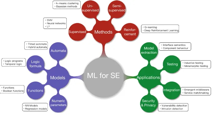
Cover illustration: Classification of key concepts of ML for software engineering. LNCS 11026, p. 5. Used with permission.
Machine learning of software artefacts is an emerging area of interaction between the machine learning (ML) and software analysis (SA) communities. Increased produc-tivity in software engineering hinges on the creation of new adaptive, scalable tools that can analyze large and continuously changing software systems. For example: Agile software development using continuous integration and delivery can require new documentation models, static analyses, proofs and tests of millions of lines of code every 24 h. These needs are being addressed by new SA techniques based on ML, such as learning-based software testing, invariant generation, or code synthesis. ML is a powerful paradigm for SA that provides novel approaches to automating the generation of models and other essential artefacts. However, the ML and SA communities are traditionally separate, each with its own agenda.
This book is a follow-up of a Dagstuhl Seminar entitled“16172: Machine Learning for Dynamic Software Analysis: Potentials and Limits” that was held during April 24–27, 2016. This seminar brought together top researchers active in these twofields to present the state of the art and suggest new directions and collaborations for future research. We, the organizers, feel strongly that both communities have much to learn from each other, and the seminar focused strongly on fostering a spirit of collaboration in order to share insights and to expand and strengthen the cross-fertilization between these two communities.
Our goal in this book is to give an overview of the ML techniques that can be used for SA and provide some example applications of their use. Besides an introductory chapter, the book is structured into three parts: testing and learning, extension of automata learning, and integrative approaches as follows.
Introduction
– The chapter by Bennaceur and Meinke entitled “Machine Learning for Software Analysis: Models, Methods, and Applications”introduces the key concepts of ML focusing on models and some of their applications in software engineering.
Testing and Learning
– The chapter by Meinke entitled “Learning-Based Testing: Recent Progress and Future Prospects” reviews the fundamental concepts and theoretical principles of learning-based techniques.
– The chapter by Walkinshaw entitled “Testing Functional Black-Box Programs without a Specification”focuses on examining test executions and informing the selection of tests from programs that do not require sequential inputs.
Extensions of Automata Learning
– The chapter by Howar and Steffen entitled“Active Automata Learning in Practice: An Annotated Bibliography of the Years 2011 to 2016”reviews the state of the art and the open challenges for active automata learning.
– The chapter by Cassel, Howar, Jonsson and Steffen entitled“Extending Automata Learning to Extended Finite State Machines” focuses on automata learning for extendedfinite state machines.
– The chapter by Groz, Simao, Petrenko, and Oriat entitled“Inferring FSM Models of Systems Without Reset”presents active automata learning algorithms that relax the assumptions about the existence of an external oracle.
Integrative Approaches
– The chapter by Hähnle and Steffen entitled“Constraint-Based Behavioral Consis-tency of Evolving Software Systems”proposes to combine glass-box analysis with automata learning to help bridge the gap between the design and implementation artefacts.
– The chapter by Alrajeh and Russo entitled “Logic-Based Machine Learning in Software Engineering” focuses on logic-based learning and its application for declarative specification refinement and revision.
While the papers in this book cover a wide range of topics regarding ML techniques for model-based software analysis, additional research challenges and related research topics still exist for further investigation.
We hope that you enjoy this book and that it will kindle your interest in and help your understanding of this fascinating area in the overlap of ML and SA. We thank the participants of the seminar for their time and their help in reviewing the chapters. Each chapter was reviewed by at least two reviewers and many went through several revi-sions. We acknowledge the support of Schloss Dagstuhl—Leibniz Center for Infor-matics and thank the whole Dagstuhl team for their professional approach that made it easy for the participants to network, to discuss, and to have a very productive seminar. Andfinally, we sincerely thank the authors for their research efforts, for their will-ingness to respond to feedback from the reviewers and editorial team. Without their excellent contributions, this volume would not have been possible.
May 2018 Amel Bennaceur
Program Chairs
Amel Bennaceur The Open University, UK
Reiner Hähnle Technische Universität Darmstadt, Germany Karl Meinke KTH Royal Institute of Technology, Sweden
Program Committee
Amel Bennaceur The Open University, UK
Roland Groz Grenoble Institute of Technology, France Falk Howar TU Dortmund and Fraunhofer ISST, Germany Reiner Hähnle Technische Universität Darmstadt, Germany Karl Meinke KTH Royal Institute of Technology, Sweden Mohammad Reza Mousavi School of IT, Halmstad University, Sweden Bernhard Steffen TU Dortmund, Germany
Introduction
Machine Learning for Software Analysis: Models, Methods,
and Applications . . . 3 Amel Bennaceur and Karl Meinke
Testing and Learning
Learning-Based Testing: Recent Progress and Future Prospects . . . 53 Karl Meinke
Model Learning and Model-Based Testing . . . 74 Bernhard K. Aichernig, Wojciech Mostowski,
Mohammad Reza Mousavi, Martin Tappler, and Masoumeh Taromirad
Testing Functional Black-Box Programs Without a Specification. . . 101 Neil Walkinshaw
Extensions of Automata Learning
Active Automata Learning in Practice: An Annotated Bibliography
of the Years 2011 to 2016 . . . 123 Falk Howar and Bernhard Steffen
Extending Automata Learning to Extended Finite State Machines . . . 149 Sofia Cassel, Falk Howar, Bengt Jonsson, and Bernhard Steffen
Inferring FSM Models of Systems Without Reset . . . 178 Roland Groz, Adenilso Simao, Alexandre Petrenko, and Catherine Oriat
Integrative Approaches
Constraint-Based Behavioral Consistency of Evolving Software Systems . . . . 205 Reiner Hähnle and Bernhard Steffen
Logic-Based Learning: Theory and Application. . . 219 Dalal Alrajeh and Alessandra Russo
Models, Methods, and Applications
Amel Bennaceur1 and Karl Meinke2(B)
1
The Open University, Milton Keynes, UK [email protected] 2
KTH Royal Institute of Technology, Stockholm, Sweden [email protected]
Abstract. Machine Learning (ML) is the discipline that studies meth-ods for automatically inferring models from data. Machine learning has been successfully applied in many areas of software engineering includ-ing: behaviour extraction, testing and bug fixing. Many more applications are yet to be defined. Therefore, a better fundamental understanding of ML methods, their assumptions and guarantees can help to identify and adopt appropriate ML technology for new applications.
In this chapter, we present an introductory survey of ML applications in software engineering, classified in terms of the models they produce and the learning methods they use. We argue that the optimal choice of an ML method for a particular application should be guided by the type of models one seeks to infer. We describe some important principles of ML, give an overview of some key methods, and present examples of areas of software engineering benefiting from ML. We also discuss the open challenges for reaching the full potential of ML for software engi-neering and how ML can benefit from software engiengi-neering methods.
Keywords: Machine learning
·
Software engineering1
Introduction
One can scarcely open a newspaper or switch on the TV nowadays without hearing about machine learning (ML), data mining, big data analytics, and the radical changes which they offer society. However, the layperson might be sur-prised to learn that these revolutionary technologies have so far had surprisingly little impact on software engineers themselves. This may be yet another case of the proverbialcobbler’s children having no shoes themselves. Nevertheless, by examining the recent literature, such as the papers published in this workshop volume, we can see small but perhaps significant changes emerging on the horizon for our discipline.
Surely one obstacle to the take-up of these exciting technologies in software engineering (SE) is a general lack of awareness of how they might be applied. What problems can ML currently solve? Are such problems at all relevant for
c
Springer International Publishing AG, part of Springer Nature 2018
software engineers? Machine learning is a mature discipline, having its origins as far back as 1950s AI research. There are many excellent modern introductions to the subject, and the world hardly needs another. However, perspectives on ML from software engineering are less common, and an introduction for software engineers that attempts to be both accessible and pedagogic, is a rare thing indeed. Furthermore, at least some of the ML methods currently applied to SE are not widely discussed in mainstream ML. There is much more to ML than deep learning.
With these motivations in mind, we will present here an introduction to machine learning for software engineers having little or no experience of ML. This material might also be useful for the AI community, to better understand the limitations of their methods in an SE context. Our focussed selection of material will inevitably reflect our personal scientific agendas, as well as the need for a short concise Chapter.
To structure this introductory material, we need some organising principles. Our approach is to focus on three questions that we feel should be addressed before attempting any new ML solution to an existing software engineering prob-lem. These are:
– What class of learned models is appropriate for solving my SE problem? – For this class of models, are there any existing learning algorithms that will
work for typical instances and sizes of my SE problem? Otherwise, is it possible to adapt any fundamental ML principles to derive new learning algorithms? – Has anyone considered a similar SE problem, and was it tractable to an ML
solution?
Let us reflect on these questions in a little more detail. As depicted in Fig.1, the presentation will be structured around three main concepts:models,methods, andapplications.
1.1 Models
A learning algorithm constructs amodel M from a givendata set D. This model represents some sort of synthesis of the facts contained in D. Most machine learning algorithms perform inductive inference, to extract general principles, laws or rules from the specific observations in D. Otherwise, learning would amount to little more than memorisation. So a model M typically contains a combination of facts (from D) and conjectures (i.e. extrapolations to unseen data).
A model may be regarded as a mathematical object. Examples of types of models (on a rough scale of increasing generality) include:
– a list of numeric coefficients or weights, (w1, . . . , wn)∈Rn, – a functionf :A→B,
– a relationr⊆B,
Fig. 1.Classification of key concepts of ML for software engineering
– a deterministic finite automaton, – a timed automaton,
– a hybrid automaton,
– a first-order mathematical structure.
An important observation at this stage is that this non-exhaustive list of model types is able to support increasingly complex and structured levels of description. Our emphasis on such precise mathematical models is because for ML, a model must be machine representable. Perhaps more importantly, models are part of the vocabulary when talking about machine learning in general.
Different methods can be used to construct different models from the same underlying data set D. This is because different abstraction principles can be applied to form different views of the same data set. Therefore, to be able to apply ML, it is fundamentally important to understand the scope and relevance of the various model types. A learned modelM never has an arbitrary structure; rather its structure, parameters and values are defined and delimited by the specific method that constructed it.
1.2 Methods
The scope and power of machine learning algorithms increases each year, thanks to the extraordinary productivity of the AI community. Therefore, what was technically infeasible a few years ago, may have changed or be about to change. This rapid pace of development is reflected in current media excitement. How-ever, the SE community needs to be more aware, on a technical level, of these changes, as well as the fundamental and unchanging theoretical limits. For exam-ple, [23] has shown that there is no learning method that can identify members of the class of all total recursive functions in the limit1.
Such negative results do not necessarily mean that ML cannot be used for your SE problem. Nor does media hype imply that you will succeed. Therefore, we believe that it is beneficial to have a deeper insight into the fundamental principles of machine learning that goes beyond specific popular algorithms.
1.3 Applications
We also believe it will be beneficial for software engineers to read about suc-cess stories in applying ML to SE. Therefore, we will try to outline some SE applications (Model extraction, testing, and component integration), where ML has already been tried with some degree of success. Scalability in the face of growing software complexity is one of the greatest challenges for SE toolmak-ers. Therefore, information (however ephemeral) about the state of the art in solvable problem sizes is also relevant.
1.4 Overview of This Chapter
In Sect.2 we give a brief overview of the major paradigms of machine learning. These paradigms (such as supervised and unsupervised learning) cut across most of the important types of models as a coarse taxonomy of methods. The number of relevant types of models for SE is simply too large to cover in a short introduc-tion such as this. Therefore, in Sect.3we present models and methods focussed around various types of state machine models. State machine models have been successfully used to solve a variety of SE problems. Our introduction concludes with Sect.4, where some of these applications are discussed. Our survey of the literature will be woven into each Section continuously.
2
Learning Paradigms
Machine learning is the discipline that studies methods for automatically induc-ing models from data. This broad definition of course covers an endless variety of subproblems, ranging from simple least-squares linear regression methods to
1
advanced methods that infer complex computational structures [33]. These meth-ods often differ in their assumptions about the learning environment, and such assumptions allow us to categorise ML algorithms in a broad way as follows.
2.1 Supervised Learning
This is the most archetypical paradigm in machine learning. The problem setting is most easily explained when the underlying model (in the sense of Sect.1.1) is a mathematical function f :A→B, however the approach generalises to other models2, such as automata.
In this setting, the learning algorithm is provided with a finite set ofnlabelled examples: i.e. a set of pairs T = {(xi, yi) ∈ A×B : 1 ≤ i ≤ n}. The goal is to make use of the example set T (also known as thetraining set) to induce a function f : A → B, such that3 f(x
i) ≡ yi for each i, (see for example [50]). Notice an implicit assumption here that the training setT corresponds to some function: i.e. for each 1≤i, j≤n ifxi =xj thenyi =yj. If this assumption is false, we must conclude that either: (i) a function model is not appropriate for the training setT, and a relational modelr⊆A×Bshould be used; (this might reflect non-determinism in the System Under Learning (SUL)) or, (ii) the training set contains measurement noise, and a function model could be used when combined with data smoothing4. Thus some domain knowledge is often
needed for the best choice of model. This situation seems to be rather typical in practise.
The task of a learning algorithm is to actually construct a concrete represen-tation off for any given training setT. This could be, for example, in terms of coefficients for a set of simple basis functions that collectively describef5.
It is natural to try to evaluate the quality off as a model. By quality, we generally mean the predictive ability of f on a data setE={(wi, zi)∈A×B: 1≤i≤m}which is disjoint fromT (often called theevaluation set). To quantify the quality of f we can for example measure the percentage of instancesisuch thatf(wi)≡zi. Of course, this is only an empirical estimate of the quality off, and care needs to be taken with the choice ofE. Generally, a larger value ofm will give greater confidence in the accuracy of the quality estimate. These two steps are illustrated in Fig.2.
A larger value ofnoften leads to a modelfwith better predictive ability on the same evaluation setE. This is because many machine learning algorithms have the property ofconvergenceover increasing data sets. However, convergence is not
2
Note that in generalAandBcan be cartesian products of sets, e.g.A=A1×. . .×An. 3
Here, the relationf(xi)≡yi means thatf(xi) is very close toyi for some suitable metric. Of course one such relation is the equality relation onB.
4
By data smoothing we mean any form of statistical averaging or filtering process, that can reduce the effects of noise. Data smoothing may be necessary even when a relational model is appropriate.
5
always theoretically guaranteed for every learning algorithm. This problem can be significant for algorithms based on optimisation methods, such as deep learning.
The domainAof all possible training and evaluation inputs is often very large or even infinite. Therefore, neither perfect training, nor perfect evaluation are usually practicable. Perfect and complete learning may not even be necessary for specific applications. An approximate model may already yield sufficient information, for example to demonstrate that a bug is present in a software system under learning.
When learning is incomplete, some kind of probabilistic statement about the quality off may be adequate. A popular approach is theprobably approximately correct (PAC) learning paradigm of [61]. This paradigm expresses the quality of f in terms of two parameters: (ε, δ), where εis the probability that f(wi) lies no further than δ from zi for each (wi, zi) ∈ E. Extensive research into PAC learning (see e.g. [36]) has shown the existence of models that are PAC learnable in polynomial time, but which cannot be exactly learned in polynomial time. So being vague may pay off!
Fig. 2.Illustrating the supervised learning paradigm
A major hurdle in applying supervised learning is often the significant effort of labelling both the training and evaluation data, in order to induce a function f with sufficient quality. Fortunately, in a software engineering context, there are situations where the system under learning itself can act as a qualified teacher that can label both training and evaluation examples.
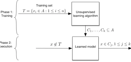
2.2 Unsupervised Learning
within the training set T, and assigns each object xi to one or more such cat-egories Cj. Thus the categoriesCj are not given a-priori. This process is illus-trated in Fig.3. Obviously, the results of unsupervised learning cannot compete with those of supervised learning. For example, in supervised learning incorrect classification is not possible as the categories are identified a-priori.
Fig. 3.Illustrating the unsupervised learning paradigm
2.3 Semi-supervised Learning
This is a pragmatic compromise between Sects.2.1and2.2. It allows one to use a combination of a small labelled example set Ts = {(x, y)} together with a larger unlabelled example set Tu ={x}. This can allow us to improve on the limited supervised learning possible withTs only, by extending the result with unsupervised learning onTu.
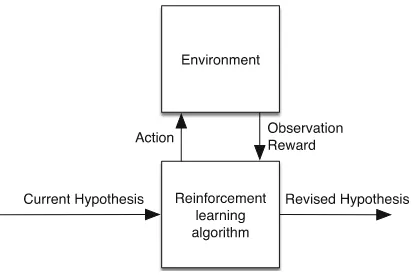
2.4 Reinforcement Learning
Reinforcement learning requires the existence of arewardmechanism that can be used to guide the learning algorithm toward a revised hypothesis as illustrated in Fig.4.
The learner is in a feedback loop with the environment with which it interacts. The learner performs an action on the environment and observes the correspond-ing reward try to get a step closer to maximiscorrespond-ing this reward. Over time, the learner optimises for the best series of actions. Q-learning [66] is an example reinforcement learning technique in which agents learn incrementally how to act optimally in controlled Markovian domains.
3
Models and Methods
Fig. 4.Illustrating the reinforcement learning paradigm
exhaustive. Some significant types of models omitted here are presented else-where in this Book. Others have been presented many times in the existing ML literature.
A general category of models which are quite natural to learn for the pur-poses of software analysis aremodels of computation for computer software or hardware. This is because such models are able to abstract away implementa-tion details (such as programming language syntax) while preserving important behavioural properties. For example, one application of machine learning for models of computation is to dynamically infer a model from runtime behaviour, and then apply a static analysis technique to this model.
In computer science, there is a long tradition of defining and studying various models of computation, including: Turing machines [30], Petri nets [53], deter-ministic finite automata (DFA) [30], pushdown automata [30], register machines [14], non-deterministic [30], probabilistic [28], and hybrid automata [4].
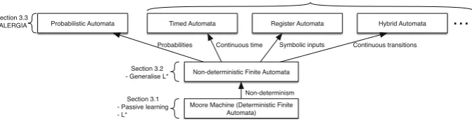
In this Chapter, we will mainly focus on different types ofautomata models. There is a rich literature around automata models that encompasses many vari-ations. The explicit computational structure of such models is able to support many of the basic aims of software analysis. Furthermore, there is the advan-tage of traceability between the training data and the learned model, which can support SE traceability and certification needs. Thus automaton learning is largely consistent with the emerging paradigm ofexplainable AI (XAI). Model traceability is often lost in other ML statistical methods.
Fig. 5.Learning automata models
Finally, we wish to compare and contrast the problem of learning across dif-ferent model classes (see Fig.5). In particular we aim to identify certain common principles and techniques that can be refined and extended to new model classes.
3.1 Deterministic Finite State Machines
Pedagogically, it is appropriate to start with the simplest automata model which is the deterministic finite state machine. Then gradually we will introduce more features associated with greater complexity both in model structure and diffi-culty of learning.
By a finite state machine (FSM), we mean a model of computation based on a finite set Q = {q0, . . . , qn} of states, and transitions (i.e. state changes) qi → qj between two states, that can occur over time. A state transition is always initiated by some input and usually returns some output. This description actually applies to many different models of computation found in the literature, including some that one would prefer to call infinite state machines. So for the purposes of studying machine learning we will need to be more precise.
A refinement of this description is that an FSM can only accept input values from afinite input alphabet Σand return values from afinite output alphabet Ω. Essentially, this means that the memory model of an FSM has a fixed and finite size. This property distinguishes the FSM model from other models, such as pushdown automata, Turing machines and statecharts [27]. The finite memory characteristic plays an important role for convergence in machine learning, as we shall see.
Supposing that from any given stateq∈Q, the same input valueσ always leads to the same next state q′ ∈ Qthen an FSM (Moore or Mealy) is said to be deterministic, otherwise it is said to benon-deterministic. Non-determinism is quite a pervasive phenomenon in software and hardware systems, especially where these are built up from loosely coupled communicating components. How-ever, because of their greater complexity, non-deterministic FSMs are harder to learn. We can consider quantifying the probabilities associated with non-deterministic choices of transitions. This leads to an even more general model termedprobabilistic automata. We shall return to these more general models in later sections of this Chapter.
In the context of models of computation, we begin then with the simplest type of learning problem, the task of learning a deterministic Moore automaton.
Definition 1. By adeterministic Moore automaton we mean a structure
A= (Q, Σ, Ω, q0, δ:Q×Σ→Q, λ:Q→Ω),
where: Q is a set of states, q0 ∈ Q is the initial state, Σ = {σ1, . . . , σk} is
a finite set of input values, Ω = {ω1, . . . , ωk′} is a finite set of output values, δ : Q×Σ →Q is the state transition function, and λ: Q →Ω is the output function.
If Q is finite then A is termed a finite state Moore automaton, otherwise A is termed an infinite state Moore automaton. Infinite state machines are useful both for pedagogical and theoretical purposes. For example, they can inspire ideas about more general learning paradigms.
The structural complexity ofA is an important parameter in studying the complexity of learning algorithms. The simplest measure here is thesizeofAas measured by the number of statesn=|Q|.
Notice that according to Definition1, a deterministic Moore automaton is a universal algebraic structure6 in the sense of [45], and this observation leads to
the subject ofalgebraic automata theory[29]. Algebraic concepts such as isomor-phisms, congruences and quotient algebras are all applicable to such structures. These algebraic concepts can be quite useful for gaining a deeper understand-ing of some of the principles of learnunderstand-ing. The followunderstand-ing insights are particularly useful.
– Structural equivalence of automata is simply isomorphism;
– The main method for automaton construction in automaton learning is the quotient automaton construction;
6
– The set of all possible solutions to an automaton learning problem can be modelled and studied as a lattice of congruences. The ordering relation is set-theoretic inclusion⊆between congruences. The maximal elements in this lattice correspond with minimal models.
Unfortunately, in a short introductory chapter such as this, we do not have space to explore this rich mathematical theory in any depth.
Deterministic Moore automata properly include deterministic finite automata (DFA) encountered in formal language theory. DFA are a special case where the output alphabet Ω is a two element set: e.g. Ω = {accept, reject}. Automaton learning algorithms found early applications in the field of natural language processing (NLP), where they were used to infer a regular grammar empirically from a corpus of texts. The sub-field of DFA learning is therefore also known as regular inference [28]. For software analysis, the generalisation from two outputs to multiple outputs Ω = {ω0, . . . ωk′} is important, and not always trivial.
Suppose that we are given as an SUL a software artifact that we wish to model and learn as a deterministic Moore automaton. We can imagine that this SUL is encapsulated within a black-box, so that we can communicate with it, without being aware of its internal structure, or even its size. This is the paradigm of black-box learning. Black-box learning is appropriate in software analysis for learning problems involving third-party, low level, dynamically changing, and even undocumented software. In practise, even when we do have access to the SUL (e.g. its source code), its explicit structure as a state machine is often far from clear. Nor is it always clear which type of state machine best captures the SUL behaviour (e.g. a deterministic or a non-deterministic machine).
To learn the SUL as a deterministic Moore machine, we observe its behaviour over time, and for this we need to be given an explicit protocol to communicate with the SUL. In practical applications, defining and implementing this protocol can be quite challenging. For example, we might communicate with the SUL in a regular synchronous fashion, or an asynchronous (event-driven) manner. We may also need to map between the abstract symbolic representation of an input setΣ and specific structured and complex input values (such as lists, queues, objects etc.). The same mapping problem applies to the outputs of the SUL andΩ.
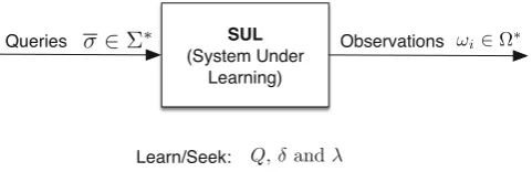
By aquery on the SUL we mean a finite string or sequenceσ=σ1, . . . , σl∈ Σ∗ of lengthl≥0 over an appropriate input alphabet Σderived from its API. Notice that even the empty stringεcan be a legitimate query for returning the initial state of the SUL on startup. If we execute the SUL on a query σthen it should return some interestingobservation. Without loss of generality, we shall assume that this observation is a string ω0, . . . , ωl ∈Ω∗, of length l+ 1. Then for each 0≤i≤l, we can assume that ωi is the result of uniformly iterating a state transition function δ, i.e.
ωi=λ(δ∗(σ1, . . . , σi)), where δ∗(ε) =q0 andδ∗(σ1, . . . , σ
We can now ask:Given an SUL, is it possible to construct complete definitions of Q,q0,δand λfor a Moore automaton model from a finite set of queries
Queries={σ1, . . . , σm}
and the corresponding set of observations
Observations={ω1, . . . , ωm}.
This is the problem ofblack-box learning a Moore automaton representation of the SUL as illustrated in Fig.6. It is clearly a supervised learning problem, in the sense of Sect.2.1. Furthermore, this problem generalises to learning other, more complex representations of the SUL. Notice that the problem specifically relates to finding a complete model that models all possible behaviours of the SUL. For certain software analysis problems, e.g. bug-finding, it may already be sufficient to construct apartial modelof the SUL, in which some SUL behaviours are missing. Notice also, that it is nota-priori clear whether a given SUL even
has a complete finite state Moore machine model. For example, the behaviours of the SUL may correspond to a push-down automaton model using unbounded memory.
Fig. 6.Illustrating black-box learning a Moore automaton
If this learning problem can be solved, we can pose further questions.
– Can we characterise a minimally adequate set of queries?
– What algorithms can be used to efficiently constructQ,q0,δandλfrom the query and observation sets?
Notice that for a behavioural analysis of the SUL, it is enough to reconstruct Q,δ andλup to structural equivalence (i.e. isomorphism). The concrete name given to each stateq∈Qdoes not impact on the input/output behaviour of the learned modelA.
3.1.1 Passive Versus Active Learning
that fits the known data. This could be because the SUL is offline, unavailable, or because we may monitor but not actively interfere with the activity of the SUL for safety reasons. This non-adaptive approach to learning is termedpassive learning.
On the other hand, it may be possible for us to generate our own queries and observe the corresponding behaviour of the SUL directly. This might be because the SUL is constantly available online to answer our queries. In this more flexible situation, new queries could be constructed according to the response of the SUL to previous queries. This adaptive approach is termedactive learning.
In the following, we will consider both of these important learning paradigms in turn.
3.1.2 Passive Automaton Learning
In passive automaton learning we are given a fixed and finite set of queries and observations for an SUL, and invited to produce our best guess about the automa-tonA(i.e. its componentsQ,q0,δandλ) that fits the known data. Passive automa-ton learning is a form of supervised learning, since we are given pairs of queries and observations, and asked to fit an optimal automaton structure to them7. Since
more than one automatonAmay fit the known data, the passive learning problem becomes an optimisation problem: how to choose the best model among a set of possible automata according to some criterion, e.g. size.
Passive learning is in some sense a simpler problem than active learning. However, the basic ideas of passive learning can be generalised to develop more interesting active learning algorithms, as we shall see later in this Section. The fundamental situation here is fairly positive. If an SUL has a representation as a finite state Moore automaton A, then the structure of A can be inferred in
Fig. 7.Illustrating passive learning of Moore machines
7
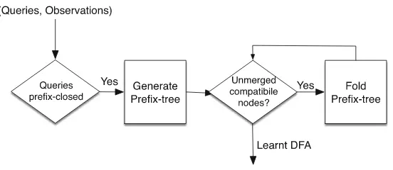
finite time from a finite number of queries. Figure7 summarises the main steps for passive learning of Moore machines which we will explain in the following.
To see this, suppose that we start to systematically enumerate and execute a sequence of queriesσ1, σ2, . . . on the SUL. For example, we could enumerate all possible input strings inΣ∗up to some maximum sizelusing the lexicographical ordering. This will produce a corresponding sequence of observationsω1, ω2, . . . from the SUL. Whatever query set is chosen, if it isprefix closed, i.e. every prefix of a query is also a query8, then we can arrange the data set of all queries and
responses into an efficient data storage structure termed a prefix tree.
Definition 2. Let Queries ⊆Σ∗ be a finite prefix closed set of queries and let
Observations⊆Ω∗ be the corresponding prefix closed set of observations for an
SUL. Theprefix tree T(Queries,Observations)is the labelled rooted tree
T(Queries,Observations) = (root,Queries, E⊆Queries2,label:Queries→Ω)
where:
1. root=ε,
2. for each(σ1, . . . , σn)∈Queries, wheren≥1,
((σ1, . . . , σn−1),(σ1, . . . , σn))∈E,
3. for each(σ1, . . . , σn)∈Queries
label(σ1, . . . , σn) =ωn+1
whereω1, . . . , ωn+1∈Observations is the SUL output for (σ1, . . . , σn).
Notice that this definition makes sense even if the set Queries is infinite, in which caseT(Queries,Observations) is a finitely branching infinite tree. In fact, if |Σ| = k then T(Queries,Observations) must have a branching degree of at mostk.
The prefix treeT(Queries,Observations) is the starting point for construct-ing all possible automaton models of the SUL, as it represents everythconstruct-ing we know about the SUL, assuming we are unable to ask further queries. Notice that although T(Queries,Observations) is a directed graph, it is not necessarily an automaton as such. In any finite prefix tree, if we start from the root and regard its edges as transitions, we eventually “jump off” when we reach a leaf node. However, interestingly enough, if Queries = Σ∗ then the infinite prefix tree T(Σ∗,Observations)isan automaton (there are no leaves to jump off). This prefix tree exactly captures the behaviour of the SUL based on perfect (infinite) infor-mation about it9. Using the fact that finite state machine behaviour is always
ulti-mately periodic, we could try to convert a prefix tree into a finite state machine model of the same data set.
8
This assumption amounts to little more than retaining, i.e. not throwing away, any observational data.
9
The most obvious way to bridge the gap between a prefix tree and an automa-ton model is to find a general method tofold any prefix tree (finite or infinite) into a finite automaton model10. The essential idea here is loop identification
by searching for finitely or infinitely repeating subtrees in the prefix tree. For finite prefix trees an important closed world assumption is at work here. If a loop cannot be shown to not exist, i.e. the loop does not contradict the available data, then we could consistently assume that the loop does exist11. In fact, it is
precisely this closed world assumption that lends inductive inference to automa-ton learning. A loop hypothesis is always an inductive inference, i.e. a hypothesis about infinitely many behaviours supported by just finite evidence.
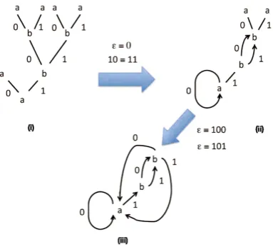
Folding a prefix tree means merging nodes in the tree in such a way that we preserve the subtrees. Figure8gives an idea of this forΣ={0,1}andΩ={a, b}. Fig (B) is obtained from the prefix tree in Fig (A) by merging the pair of nodes ε and 0 (giving a loop) and the pair 10 and 11 (giving a path join). Following this, in the second step Fig (C) is obtained from Fig (B) by merging the pairε and 100 (giving a loop), as well as the pair εand 101 (giving a loop).
Clearly, after we have merged two nodesv1, v2∈Queriesthey share all their entry and exit paths afterwards through the merged nodes12. Most importantly,
if we merge two nodes v1, v2 ∈ Queries which lie on the same path from the root13, then this always introduces a loop or cycle into the resulting directed
graph. For the result of merging to be well defined, the nodesv1andv2must be compatible in the following sense.
Definition 3. Let
T(Queries,Observations) = (root,Queries, E⊆Queries2,label:Queries→Ω)
be a prefix tree. A pair of nodes v1, v2∈Queries is said to be compatibleif the sub-trees rooted at v1 andv2 are consistent with each other, i.e. for every suffix
s∈Σ∗, ifv1.s∈Queries andv2.s∈Queries then
label(v1.s) =label(v2.s).
We write v1≃v2 ifv1 and v2 are compatible.
The consistency condition in Definition3ensures that if we merge nodesv1and v2then they do not contradict each other in the resulting merged graph. This is summarised by the fact that for anyσ∈Σwe have14:
v1≃v2 =⇒ v1.σ≃v2.σ (1)
10
The fundamental principle of initiality forT(Σ∗,Observations) says that such folding is always possible.
11
For active learning, counterfactual evidence may eventually emerge that destroys the loop hypothesis, but in passive learning this is not possible.
12
Merging is a little complicated to define graph theoretically, so we leave it to the reader as an exercise!
13
Thenv1 is a prefix ofv2or vice versa. 14
Fig. 8.A prefix tree folded in two steps with four node merges
Compatibility is a necessary condition for merging two nodesv1andv2, since the merged graph must include the information carried in both subtrees. However, compatibility is not a sufficient condition to successfully derive an automaton from the prefix tree by folding.
To see this, consider that the compatibility relation≃, is clearly reflexive i.e. v ≃ v and symmetric i.e. v1 ≃ v2 → v2 ≃ v1. However, compatibility is not always transitive, i.e. in general v1 ≃ v2 and v2 ≃ v3 do not imply v1 ≃ v3. This is because in general v1, v2 and v3 will have disjoint subtrees that need not be mutually consistent. Therefore: (i) the order in which we merge subtrees is important, (ii) different merge orders will lead to different (non-isomorphic) automaton models from the same data set, and (iii) some models may be prefer-able to others (e.g. in terms of size).
We can now express some necessary constraints on subtree folding for prefix trees in terms congruence properties.
Definition 4. Let
T(Queries,Observations) = (root,Queries, E⊆Queries2,label:Queries→Ω)
be a prefix tree.
1. By acongruenceonT(Queries,Observations)we mean an equivalence rela-tion≡on the set Queries such that for anyp, q∈Queries and anyσ∈Σ, if
p.σ∈Queries andq.σ∈Queries then
p≡q =⇒ p.σ≡q.σ.
2. A congruence≡isconsistentif, and only if, for anyp, q∈Queries, ifp≡q
3. A congruence ≡isclosed if, and only if, for any queryp∈Queries which is a leaf node in the prefix treeT(Queries,Observations)there exists a non-leaf
q∈Queries such that
p≡q.
Based on the two first items, we can infer that congruence implies compatibility,
p≡q =⇒ p≃q.
However, a consistent congruence has stronger properties than compatibility as it is transitive. This means it consistently resolves conflicting node merges. Finally, the closure condition (the third item in Definition4) rectifies the problem that the leaves of finite prefix trees are not closed under state transitions.
Now given a closed consistent congruence on a prefix tree we can construct a structure that is “almost” an automaton.
Definition 5. Let
T(Queries,Observations) = (root,Queries, E⊆Queries2,Queries→Ω)
be a prefix tree, and let ≡ be a closed consistent congruence on T(Queries,
Observations). We define thequotient structure
T(Queries,Observations)/≡
= (Q, Σ, Ω, q0, δ:Q×Σ →Q, λ:Q→Ω)
as follows15.
1. For the state set:
Q ={p/≡ :p.σ∈Queries for some σ∈Σ}
wherep/≡is the equivalence class ofpw.r.t.≡. 2. For the initial state:q0=ε/≡,
3. For anyp∈Queries and σ∈Σ, ifp.σ∈Queries then
δ(p/≡, σ) =p.σ/≡,
otherwiseδ(p/≡, σ) is undefined. 4. For anyp.σ∈Queries
λ(p/≡) =label(p).
We meet the above construction many times in automaton learning. It appears again when we study active learning, and in modified forms when learn-ing other types of automaton. The quotient structure defined above isalmost an
15
automaton, but for one small problem: the query set Queries may not contain enough information to define every transition. In this case, the state transition function δ is a partial function that is not defined on every state and input value. When we look into this problem more deeply, we realise that the query set may not even have enough information to define every state! So what kind of guarantee can we give about passive learning?
For the first time in this Chapter, but not the last, we must consider the
correctness problem for a learning algorithm. Here we view passive learning as essentially a method for the construction of some closed consistent congruence from which we can concretely build an automaton as a quotient structure. Are there necessary and sufficient conditions on the underlying query set, such that passive learning is guaranteed to yield a quotient structure that: (i) is guaran-teed to be a fully defined automaton, and (ii) is behaviourally equivalent to the SUL? Surprisingly (when compared with other paradigms of machine learning) complete and correct passive learning can be guaranteed when we have sufficient behavioural information about the SUL.
Definition 6. Let
A= (Q, Σ, Ω, q0, δ:Q×Σ→Q, λ:Q→Ω),
be a deterministic Moore automaton.
1. Let q ∈ Q be any state. By an access string for q, we mean any string
σ∈Σ∗ such thatδ∗(q0, σ) =q.
2. Letq, q′∈Qbe any states. By adistinguishing stringforqandq′, we mean
any stringσ ∈ Σ∗ such thatλ(δ∗(q, σ)) = λ(δ∗(q′, σ)). We say that qandq′
aredistinguishableif there exists a distinguishing string forqandq′. For a pair of different states q and q′ in A, a distinguishing string σ is not guaranteed to exist. But it must exist if there is no automaton that is both strictly smaller thanAand behaviourally equivalent toA.
Theorem 1. Correctness Theorem for Passive Learning.
Suppose that the SUL behaviour can be precisely described by a deterministic Moore automaton,
A= (Q, Σ, Ω, q0, δ:Q×Σ→Q, λ:Q→Ω).
Let Queries⊆Σ∗ be a set of queries such that:
1. For every stateq∈Q, Queries contains an access stringσq∈Σ∗ forq.
2. For every distinguishable pair q, q′ ∈Q of states, Queries contains bothσ q.δ
andσq′.δ, whereδ∈Σ∗ is a distinguishing string for q, q′.
3. For every state q∈Q, and for each inputσ∈Σ, Queries contains the query
σq.σ.
Then for any closed consistent congruence ≡ on T(Queries,Observations)
Proof. Exercise.
To illustrate the Correctness Theorem1 for Passive Learning, suppose that we take the final Fig.8(iii) as the Moore automaton to be learned. Then the prefix tree of Fig.8(i) satisfies the three properties of Theorem1. Furthermore, there exists a closed consistent congruence ≡containing the equivalences (node identifications)ε≡0,10≡11, ε≡100 andε≡101. Then the resulting quotient automaton derived from Fig.8(i) using≡is isomorphic with Fig.8(iii). In other words, passive learning applied to Fig.8(i) successfully gives Fig.8(iii). It should be obvious that no larger prefix tree than Fig.8(i) is necessary to learn Fig.8(iii). An important point to emphasise here is that in general there are many dif-ferent congruences≡on any specific prefix treeT(Queries,Observations). Differ-ent congruences will lead to structurally differDiffer-ent (i.e. non-isomorphic) quotiDiffer-ent automata. Nevertheless, each quotient automaton T(Queries,Observations)/≡ will exhibit all of the behaviours observed in the original data set ofQueriesand
Observations.
From this important observation, we are motivated to further refine model construction by choosing the “best” model according to some principle such as Occam’s razor (the principle of parsimony). The best model might be considered to be a minimum state automaton. However [24] has shown that the problem of finding a minimum state DFA compatible with a given dataset is NP Hard. Thus all known algorithms for this problem require exponential time for some inputs.
Considering the fact that there is not usually a single maximum congruence, in general, there are several maximal16 congruences and it is natural to choose
from among these. Other criteria can be used to refine this choice.
One additional criterion is known as theevidence driven approach. Here we successively merge node pairsv1, v2for which the compatibility evidence is great-est. This corresponds to choosing the largest possible subtrees, which have the greatest power to refute a merge. It also corresponds intuitively to making the least controversial hypotheses about the structure of the SUL. Algorithms based on this approach have performed well in benchmarking studies [38].
Obviously, passive automaton learning converges as a finite model construction from a fixed finite data set, when correctly implemented. Notice however, that in terms of query set size, Theorem1 implies that passive automaton learning also converges in the limit. For once we have accumulated enough access strings, single input extensions to these, and distinguishing strings, then further querying cannot destroy any of these conditions.
Now the only question remains, short of exhaustive querying, how can we compile a set of queries that satisfies Conditions 1, 2 and 3 of Theorem1, and how can we build the appropriate congruence≡? This question is best answered by the subject of active automaton learning, which we consider next.
16
3.1.3 Active Automaton Learning
In passive automaton learning we are given a dataset of queries and observations about the SUL and asked to construct an automaton model which best fits this dataset. The accuracy of any model will be limited by the number of queries in the dataset. Theorem1 even suggests that we will obtain a behaviourally incomplete model of the SUL if key queries are missing from the dataset.
In active automaton learning, these problems can be circumvented since the training regime is more liberal. Active learning means that at any time in the learning process we can supplement the existing dataset by asking new queries which the SUL must answer. This also means we can focus on heuristics for active query generation that could speed up the learning process. From the study of active learning, it becomes clear that neither exhaustive nor random querying are good heuristics, since both methods generate many redundant queries.
Active automaton learning is again a form of supervised learning, since query and observation pairs are involved. Many active automaton learning algorithms have been published in the literature. Useful surveys include [9,28,68]. In this section, we will look at a well-known and widely used active learning algorithm L* originating17 in [6]. This algorithm works quite well on small examples,
though it can generate an excessive number of queries on larger case studies. Nevertheless, it is easy to understand and implement, while it involves simi-lar principles to those used in more efficient algorithms. Under the assumption that we can efficiently detect differences between the learned automaton and the SUL, the L* algorithm can be mathematically proven to completely learn an automaton in polynomial time. One can even prove that L* constructs the unique minimum state automaton that is behaviourally equivalent to the SUL, which is in itself a useful property18.
We begin by clarifying the experimental protocol for active learning. If there is a way to bring the SUL back to its initial stateq0after each individual queryσi then the SUL is said to satisfy thereset assumption. This assumption allows us to isolate the effects of each query from the next. Without the reset assumption, in black-box learning we have no way of knowing what state the SUL is left in after it processes query σi. This unknown SUL state becomes the new initial state for processing the next queryσi+1. Thus, to query the SUL without the reset assumption is effectively to query it using one single long query. Learning algorithms exist (see the Chapter by Groz et al. [54]) that do not require the reset assumption. However, such algorithms tend to be complex. For applying L*, and many other active automaton learning algorithms, we assume that the reset assumption holds.
17
We actually present a simple generalisation of L* to an arbitrary output alphabet Ω. This algorithm is termed L*Mealy and first appeared in [34] where it was applied to Mealy machines.
18
The basic idea of all active automaton learning algorithms is to find a way to identify incompleteness in a dataset. By an incomplete dataset, we mean a dataset of queries and observations that does not allow us to unambiguously infer a behaviourally equivalent SUL model. If a specific incompleteness can be identified in the dataset then this can be used to actively generate a new query. Executing this query on the SUL will then bring the entire dataset somewhat closer to completeness. By iterating this process of identifying and resolving dataset incompleteness (hopefully) eventually learning will be complete.
For many active automaton learning algorithms, a mathematical analysis can be used to show that learning will always eventually terminate yielding a behaviourally equivalent automaton model. Such a result is called aconvergence theorem for the learning algorithm in question. Active automaton learning is rather rich both in algorithms and in convergence theorems. This can be con-trasted with other branches of ML where convergence cannot always be guar-anteed, e.g. deep learning. On the other hand, the datasets necessary to achieve complete learning may be infeasibly large. Good methods for approximate learn-ing are an important open problem.
The L* algorithm has its own specific active querying heuristics. For L*, incompleteness is divided into two kinds: (i) incompleteness due to not being able to immediately generate a model, and (ii) incompleteness due to lacking a full set of queries (access and distinguishing strings) for the SUL. While type (ii) incompleteness is very intuitive, type (i) incompleteness is rather technical, and will be further broken down into more detailed requirements.
A good starting point for presenting L* is to define the underlying data structure used to identify type (i) incompleteness in the query set. This is more complex than the prefix tree (Definition2) we saw earlier in passive learning. However, it is not unrelated in content.
Suppose thatQueries⊆Σ∗andObservations⊆Ω∗ are the current dataset of queries and observations of the SUL. The main data structure for L* is a two dimensional tableT. The table entries inT are output values fromΩ. The table rows and columns are indexed by strings over Σ∗. However, the table T is allowed to expand dynamically over time, as we incrementally learn the SUL using new queries. One difficulty in presenting the L* algorithm is to explain this expansion process forT.
At any stage in the execution of L*, there are three distinguished table index-ing sets:
– a set PrefixesRed ⊆ Σ∗ of red prefixes which is a prefix-closed set of input strings,
– a set PrefixesBlue = PrefixesRed.Σ of blue prefixes which is a prefix-closed set of input strings that extends each red prefix with one extra input symbol (chosen over all possible input symbols inΣ),
We follow a common pedagogy here of distinguishing betweenred andblue pre-fixes19. The rows of T are indexed by red and blue prefixes from the set
PrefixesRed∪PrefixesBlue,
and the columns ofT are indexed by suffixes from the setSuffixes.
How are SUL output values stored as table entries ofT? Let us writeT[p, s] for the table entry ofT in rowpand columns. We can concatenate prefixpwith suffixsyielding the query string
p.s=p1, . . . , pi, s1, . . . , sj.
Now the behaviour of the SUL on p.swill already be known if p.s is a prefix of some q ∈ Queries. In this case we have a recorded SUL observation ω = ω0, . . . , ωi+j corresponding to p.s. In particular, we know the value of
ωi+j =λ(δ∗(q0, p.s))
(whereδ∗ is the iterated state transition function defined above) and this value ωi+j is placed in the table entryT[p, s].
Suppose on the other hand thatp.s is not currently a member ofQueries. Then we can query the SUL usingp.sas an active query and observe the value of ωi+j =λ(δ∗(q0, p.s)). This value is placed in the table at T[p, s]. Thus, the most basic form of active querying in L* comes from filling in missing entries in the two dimensional tableT. We call thesetable-entry queries.
The basic principle for inferring a Moore automaton from a completely filled-in two dimensional table T is as follows: if T[p, s] = T[q, s], for some suffix s then the input stringspandqcannot possibly reach the same state in the SUL, provided that the SUL is deterministic20. In other words, the subtrees atpand
q in the corresponding prefix tree (having the same query content as T) are incompatible.
It follows that if any two rows inT differ at all, say T[p]=T[q] then pand q must access distinct states in the SUL. Therefore, we can partition the red prefix setPrefixesRed into equivalence classes of row-identical red prefixes using T. As a concrete representative of each equivalence class, typically the shortest access string is chosen as a state name.
Table-entry queries are the primary source of type (i) queries. But how is it that gaps ever arise in the tableT? This is due to the already hinted expansion of T that takes place during the learning process. To be able to directly and unambiguously construct an automaton model fromT, the structure ofT must satisfy two very specific technical properties.
19
In model construction, red prefixes are needed to represent states, while blue prefixes are needed for defining transitions. According to our definition, a prefix can be both red and blue, but this is not problematic.
20
Definition 7. Let
T :PrefixesRed∪PrefixesBlue×Suffixes→Ω
be a two dimensional table.
(i) We say that T is closed if for each red prefix p ∈ PrefixesRed and input σ ∈ Σ there exists a red prefixq ∈ PrefixesRed such that the rows T[p.σ] and T[q]inT are identical, i.e.T[p.σ] =T[q].
(ii) We say that T is consistent if for any red prefixes p, q ∈ PrefixesRed, if T[p] =T[q] then for all inputsσ∈Σ we have T[p.σ] =T[q.σ]21.
Notice that blue prefixes are necessary in both Definition7(i) and (ii) since even if a prefix pis red, the prefixp.σ may be blue. This technical need for closure and consistency inT leads to two different sub-algorithms for generating active queries fromT as follows.
ALGORITHM 1.makeConsistent()
1 findp, q∈Prefixes
Red,σ∈Σ
2 ands∈Suffixessuch that 3 T(p) =T(q)and
4 T(p.σ, s)=T(q.σ, s)
5 letSuffixes:=Suffixes∪ {σ.s}// suffix set extension 6 extendTtoPrefixes
Red∪PrefixesBlue×Suffixes
7 using table-entry queries.
ALGORITHM 2.makeClosed()
1 findp∈Prefixes
Red andσ∈Σsuch that
2 T(p.σ)=T(q)for allq∈Prefixes
Red
3 letPrefixes
Red:=PrefixesRed∪ {p.σ}// red prefix set extension
4 letPrefixes
Blue:=PrefixesBlue∪ {p.σ} ×Σ// blue prefix set extension
5 extendT toPrefixes
Red∪PrefixesBlue×Suffixes
6 using table-entry queries
Using the concepts of closure and consistency, we can now make precise the basic iteration step in L* for learning a new automaton modelMn+1, given that we have previously learned Mn.
21
ALGORITHM 3.getNextHypothesis(equivalenceQuery ∈Σ∗)
1 Prefixes
Red:=PrefixesRed∪P ref ixClosure(equivalenceQuery)
2 Prefixes
Blue:=PrefixesBlue∪ {equivalenceQuery} ×Σ
3 Suffixes:=Suffixes∪suffixClosure(equivalenceQuery) 4 extendT toPrefixes
Red∪PrefixesBlue×Suffixes
5 using table-entry queries 6
7 whileTis not closed orTis not consistent do 8 if!consistent(T)makeConsistent()
9 else if!closed(T)makeClosed()
The routinegetNextHypothesis()adds a single new queryequivalenceQuery to the existing query set and extends the tableTwith the appropriate new red and blue prefixes and suffixes derived fromequivalenceQuery. All new entries in the resulting expanded tableT are filled in by table-entry queries. Following this, the structure of the newly expanded tableTis analysed for failure of closure or consis-tency. The remedial measuresmakeClosed()andmakeConsistent()may further expand the tableT. Note that if the SUL is behaviourally equivalent to an automa-ton then the while loop ingetNextHypothesis()will eventually terminate. Upon termination, i.e. whenT is both closed and consistent, then the construction of modelMn+1can be carried out with the following routine.
ALGORITHM 4.mooreSynthesis()
1 // Choose state representatives as smallest red prefixes 2 Q={p∈Prefixes
Red:∀q∈PrefixesRed, q < p→T[p]=T[q]}
3 q0=ε
4 foreachp∈Q,λ(p) =T[p, ε] 5 foreachp∈Qdo
6 foreachσ∈Σdo
7 δ(p, σ) =qifq∈QandT[p.σ] =T[q] 8 returnA= (Q, Σ, q0, δ, λ)
This algorithm may be compared with the quotient automaton construction of Definition5 which it makes more concrete.
As already observed, red prefixes form the basis for the state setQofMn+1. In Algorithm4, the first member p of each red prefix equivalence class under some linear ordering22<is chosen to be the state representative. Note that the
empty stringεwill always be a red prefix, but needs to be the least member of its
22
equivalence class [ε]. Thenεis the appropriate access string for the initial state q0in Mn+1. It is easy to see thatλ:Q→Ωis mathematically well defined as a function. The reader should observe how the closure and consistency conditions onT ensure that the state transition mapδis also mathematically well defined.
– For each red prefixp∈Qand inputσ∈Σ there exists red prefixq∈Qthat is row equivalent to the (possibly blue) prefix p.σ by closure ofT. Thus the value ofδ(p, σ) isdefined.
– By consistency ofT, the rowT[p.σ] and hence the value ofδ(p, σ) isuniquely
defined.
We can construct the initial hypothesis automatonM0, in the sequence of models M0, M1, . . ., by calling getNextHypothesis() on the empty string as follows.
ALGORITHM 5.getInitialHypothesis()
1 Prefixes
Red:=∅// emptyset
2 Prefixes
Blue:=∅
3 Suffixes:=∅
4 return getNextHypothesis(ε)
Finally, we can describe the complete L* algorithm. This algorithm combines getInitialHypothesis()withgetNextHypothesis()and a stopping criterion for iterative model generation M0, M1, . . . based on equivalence checking. This equivalence checking of each learned modelMiwith the SUL is the source of the active type (ii) queries mentioned previously.
ALGORITHM 6.LStar(SUL)
1 varPrefixes
Red
2 varPrefixes
Blue
3 varSuffixes 4 varT :Prefixes
Red∪PrefixesBlue×Suffixes→Ω // table
5 varA
6 A :=getInitialHypothesis()
7 while( !equivOracle(A, SU L).equivalent)do
8 A :=getNextHypothesis(equivOracle(A, SUL).equivalenceQuery) 9 endwhile
10 returnA
The desired behaviour of the equivalence oracle is specified as follows.
Definition 8. Given two parameters consisting of a Moore automatonA and a system under learning SU L, an equivalence oracle on A andSU L returns two parameters:equivalent∈ {true, f alse}and equivalenceQuery∈Σ∗.
1. For the return parameterequivalent:
equivalenceOracle(A, SU L).equivalent=
true if ∀p∈Σ∗A(p) =SU L(p)
f alse otherwise (2)
2. For the return parameterequivalenceQuery:
equivalenceOracle(A, SU L).equivalenceQuery=
p if A(p)=SU L(p) null otherwise (3)
Designing an implementation of an equivalence oracle can be somewhat prob-lematic. Firstly, the SUL is a black-box, so there is no direct way to compare its internal structure with the state transition structure of Mi. Black-box equiva-lence checking algorithms, that are independent of the internal structure of the SUL are for example the Vassilevsky-Chow algorithm [15,62]. Another approach is to usestochastic equivalence checking, (see e.g. [6]) based on a random sample of input sequences. Here the challenge is to identify an appropriate sample size and length bound for the random input string set. Stochastic equivalence check-ing might seem like machine learncheck-ing uscheck-ing random queries, and in some sense this is true. However, the percentage of random queries in the overall query set will be very small, usually less than 1%. An advantage of stochastic equivalence checking is its connection to the PAC learning paradigm cited previously [61].
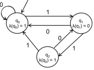
Fig. 9.Simple DFA for learning
Table 1.Closed: no, consistent: yes Table 2.Closed: yes, consistent: yes
but not closed. A single call to makeClosed() produces Table2 which is both closed and consistent. At this point, the initial modelM0can be constructed by a call tomooreSynthesis().
The initial model M0 is depicted in Fig.10. Clearly, this model replicates some but not all of the behaviour of the DFA in Fig.9. A call to the equivalence oracle gives the following results:
equivalenceOracle(M0, SU L).equivalent=f alse,
equivalenceOracle(M0, SU L).equivalenceQuery= 110.
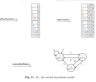
Adding the equivalence query 110 to Table2 by calling getNextHypothesis (110)gives Table3.
Table 3.Closed: yes, consistent: no Table 4.Closed: yes, consistent: yes
Fig. 11.M1, the second hypothesis model
Table3 is closed, but there are two inconsistencies, since T(ε) =T(11) but (1) T(1) = T(111), and (2) T(0) = T(110). So after two separate calls to makeConsistent(), we obtain Table4.
Now Table4 is closed and consistent, so the next model M1 can be con-structed by another call tomooreSynthesis()and is depicted in Fig.11. Notice that in Table4there are four red prefixes, but two of these, 1and110, are row equivalent. Therefore, model M1 has just three distinct states.
NowM1 is structurally isomorphic with, and therefore behaviourally equiva-lent to, the SUL in Fig.9. According to the theory of L*, structural isomorphism implies that Fig.9 was a minimum state DFA to begin with.
A convergence result (i.e. a statement of both correctness and termination) for the L* learning algorithm is the following.
Theorem 2. Convergence Theorem for L*. Suppose that the SUL behaviour can be precisely described by a DFA and let A be a minimal representation of this DFA. Then the L* algorithm eventually terminates and outputs a DFA isomor-phic toA. Moreover, ifnis the number of states of Aandmis an upper bound on the length of any counterexample provided by the equivalence checker, then the total running time of L* is bounded by a polynomial in mandn.
We end this section with an important observation about both passive and active learning of deterministic finite state machines. Our theoretical exposition and the case study above both reveal the important fact that every feature of the final learned modelMiistraceableback to behaviours of the SUL. Therefore they can be reproduced and independently confirmed even after the learning session has terminated. This fact will be important in the future for software engineering applications, where traceability between conclusions and their evidence may be legally required, e.g. by certification processes such as ISO 26262 [1].
One reason for traceability in automaton learning is the absence (for better or worse) of any statistical learning methods, which smooth the dataset. Said simply: what you get is what you see (WYGIWYS). Another reason for trace-ability is the explicit state space structure and construction of the model M. There are other ML techniques which can also learn temporal behaviours, for example, recurrent and deep neural networks. However, for software engineer-ing, such algorithms may be problematic in the sense that they lack traceability between the learned model and the original SUL.
3.2 Non-deterministic Finite State Machines
In the context of software engineering, given an arbitrary black-box SUL, it may be difficult to be certain that its behaviour is entirely deterministic. On the contrary, for many large-scale distributed systems that we would like to model, we can often be confident of extensive non-deterministic behaviour. The ML models and methods of Sect.3.1 have a restricted value in this case. For example, L*, as we have described it, would record the first observed behaviour of a non-deterministic SUL in the table T and simply ignore later alternative behaviours. This yields a partial model that will lack any alternative behaviours. Clearly, it would be appropriate here to learn a more general non-deterministic automaton model.
Definition 9. By a non-deterministic Moore automaton we mean a structure
A= (Q, Σ, Ω, q0, δ:Q×Σ×Q, λ:Q→Ω),
where: Q = {q1, . . . qn} is a set of states, q0 ∈ Q is the initial state, Σ = {σ1, . . . , σk} is a finite set of input values,Ω ={ω1, . . . , ωk′} is a finite set of
output values, δ:Q×Σ×Q is the state transition relation, andλ:Q→Ω is the output function.
The main difference in Definition9 compared with Definition1 of Sect.3.1.3is that the state transition relation δ allows us to capture each of the multiple states q′ ∈Q to whichA can transition from any given stateq ∈Qunder the same input σ∈Σ.