Kvazaar HEVC videokooderin pakkaustehokkuuden ja suorituskyvyn optimointi

(1)

ARTTU YLÄ-OUTINEN

CODING EFFICIENCY AND COMPLEXITY OPTIMIZATION

OF KVAZAAR HEVC ENCODER

Master of Science thesis

Examiner: Ass. Prof. Jarno Vanne Examiner and topic approved on 30th November 2017

(2)

I

ABSTRACT

ARTTU YLÄ-OUTINEN: Coding Efficiency and Complexity Optimization of Kvazaar HEVC Encoder

Tampere University of Technology Master of Science thesis, 46 pages June 2018

Master’s Degree Programme in Information Technology Major: Software Engineering

Examiner: Ass. Prof. Jarno Vanne

Keywords: High Efficiency Video Coding (HEVC), Kvazaar HEVC encoder, video coding, coding efficiency, computational complexity

Growing video resolutions have led to an increasing volume of Internet video traffic, which has created a need for more efficient video compression. New video coding standards, such as High Efficiency Video Coding (HEVC), enable a higher level of compression, but the complexity of the corresponding encoder implementations is also higher. Therefore, encoders that are efficient in terms of both compression and complexity are required.

In this work, we implement four optimizations to Kvazaar HEVC encoder: 1) uni-form inter and intra cost comparison; 2) concurrency-oriented SAO implementation; 3) resolution-adaptive thread allocation; and 4) fast cost estimation of coding co-efficients. Optimization 1 changes the selection criterion of the prediction mode in fast configurations, which greatly improves the coding efficiency. Optimization 2 re-places the implementation of one of the in-loop filters with one that better supports concurrent processing. This allows removing some dependencies between encoding tasks, which provides more opportunities for parallel processing to increase coding speed. Optimization 3 reduces the overhead of thread management by spawning fewer threads when there is not enough work for all available threads. Optimiza-tion 4 speeds up the computaOptimiza-tion of residual coefficient coding costs by switching to a faster but less accurate estimation.

The impact of the optimizations is measured with two coding configurations of Kvazaar: the ultrafast preset, which aims for the fastest coding speed, and the veryslow preset, which aims for the best coding efficiency. Together, the introduced optimizations give a 2.8×speedup in theultrafast configuration and a 3.4×speedup in theveryslow configuration. The trade-off for the speedup with theveryslowpreset is a 0.15 % bit rate increase. However, with the ultrafast preset, the optimizations also improve coding efficiency by 14.39 %.

(3)

II

TIIVISTELMÄ

ARTTU YLÄ-OUTINEN: Kvazaar HEVC videokooderin pakkaustehokkuuden ja suorituskyvyn optimointi

Tampereen teknillinen yliopisto Diplomityö, 46 sivua

Kesäkuu 2018

Tietotekniikan DI-tutkinto-ohjelma Pääaine: Ohjelmistotuotanto Tarkastaja: Ass. Prof. Jarno Vanne

Avainsanat: High Efficiency Video Coding (HEVC), Kvazaar HEVC videokooderi, videon-pakkaus, pakkaustehokkuus, laskennallinen vaativuus

Digitaalisen videon resoluutioiden kasvaessa Internetin videodataliikenne on lisään-tynyt, mikä puolestaan on luonut tarpeen tehokkaammalle videonpakkaukselle. Uu-det videokoodausstandardit, kutenHigh Efficiency Video Coding (HEVC), mahdol-listavat tehokkaamman videonpakkauksen mutta kasvattavat myös videokooderien vaatimaa laskentatehoa. Tavoitteena onkin kehittää videokooderi, joka pystyy pak-kaamaan videota sekä tehokkaasti että nopeasti.

Tässä työssä toteutetaan videonpakkausohjelmisto Kvazaariin neljä optimointia: 1) kustannusten yhdenmukainen vertailu; 2) rinnakkaisuutta tukeva SAO-toteutus; 3) videon resoluution mukaan säätyvä säikeiden määrä; ja 4) nopea jäännösvirheen kus-tannuksen arviointi. Optimointi 1 muuttaa valintakriteeriä kuvan sisäisen ja kuvien välisen ennustuksen valinnassa, mikä parantaa pakkaustehokkuutta merkittävästi. Optimointi 2 muokkaa SAO-suotimen toteutusta tukemaan paremmin rinnakkaista laskentaa. Tämän ansiosta joitakin riippuvuuksia koodaustyökalujen välillä voidaan poistaa, mikä mahdollistaa rinnakkaisuuden lisäämisen nopeuttaen pakkausta. Op-timointi 3 vähentää säikeiden hallintaan kuluvaa aikaa käynnistämällä vähemmän säikeitä silloin, kun useammalle säikeelle ei ole tarpeeksi käyttöä. Optimointi 4 no-peuttaa jäännösvirheen koodaamiseen vaadittavan bittimäärän laskemista hyödyn-täen nopeampaa mutta vähemmän tarkkaa arviointimenetelmää.

Muutosten vaikusta mitataan seuraavilla Kvazaarin koodausasetuksilla: ultrafast, joka pyrkii mahdollisimman korkeaan suoritusnopeuteen, ja veryslow, joka pyrkii mahdollisimman hyvään pakkaustehokkuuteen. Optimoinneilla saavutetaan yhteen-sä 2,8×nopeutusultrafast-asetuksilla ja 3,4×nopeutusveryslow-asetuksilla. Nopeu-tus kasvattaa veryslow-asetuksilla bittimäärää 0,15 %, mutta ultrafast-asetuksilla muutokset parantavat myös pakkaustehokkuutta 14,39 %.

(4)

III

PREFACE

This thesis was written as a part of research conducted in the Laboratory of Pervasive Computing at Tampere University of Technology during the years 2017–2018. First and foremost, I would like to thank my supervisorJarno Vannefor his helpful advice and feedback on this thesis. I would also like to thank all contributors to the Kvazaar project.

Finally, I would like to give a heartfelt thanks to my parents Lea and Kai for all their support during my studies.

Tampere, June 2018

(5)

IV

LIST OF FIGURES

2.1 Overview of the data flow in Kvazaar encoding process . . . 6

2.2 An example of a CTU split into CUs and the corresponding quadtree 7 2.3 Partition modes available in HEVC . . . 8

2.4 Reference pixels for intra prediction . . . 9

2.5 Locations of the spatial and temporal AMVP candidates . . . 11

4.1 Visualization of parallel encoding . . . 28

4.2 Intra-frame and inter-frame dependencies for a single CTU . . . 29

4.3 CTU split into four regions for in-loop filters . . . 30

4.4 Intra-frame CTU dependencies in a single frame . . . 34

4.5 Parallel coding of three consecutive frames with OWF . . . 34

(8)

VII

LIST OF TABLES

2.1 Kvazaar coding tools with the analyzed presets . . . 16

3.1 Properties of the test computer . . . 20

3.2 Details of the test sequences . . . 21

4.1 Kvazaar CU size and mode usage . . . 23

4.2 x265 CU size and mode usage . . . 23

4.3 Kvazaar CU size and mode usage with intra skip disabled . . . 23

4.4 BD-rate for different inter cost multiplier values . . . 24

4.5 BD-rate and speedup for different intra skip threshold values . . . 26

4.6 Effect of Optimization 1 on BD-rate and complexity . . . 26

4.8 Relative speed for different numbers of threads and OWF . . . 33

4.9 Comparison of the selection algorithms for the number of threads and OWF . . . 36

4.10 Effect of Optimization 3 on complexity . . . 37

5.1 Optimized Kvazaar, Turing encoder, and x265 compared with the original Kvazaar with the fastest presets . . . 40

5.2 Optimized Kvazaar, Turing encoder, and x265 compared with the original Kvazaar with the slowest presets . . . 41

(9)

VIII

LIST OF ABBREVIATIONS AND SYMBOLS

AMVP Advanced motion vector prediction

AVC Advanced Video Coding

BD-rate Bjøntegaard-delta bitrate BMA Block matching algorithm

CABAC Context-adaptive binary arithmetic coding CPU Central processing unit

CTU Coding tree unit

CU Coding unit

DCT Discrete cosine transform DST Discrete sine transform FME Fractional motion estimation GOP Group of pictures

HEVC High Efficiency Video Coding HEXBS Hexagon-based search

HM HEVC test model

IEC International Electrotechnical Commission ISO International Organization for Standardization ITU International Telecommunication Union

ITU-T ITU Telecommunication Standardization Sector JCT-VC Joint Collaborative Team on Video Coding LGPL GNU Lesser General Public License

ME Motion estimation

MPEG Motion Picture Experts Group

MSE Mean squared error

MV Motion vector

MVP Motion vector predictor OWF Overlapped wavefronts PSNR Peak signal-to-noise ratio

PU Prediction unit

QP Quantization parameter RD-cost Rate–distortion cost

RDOQ Rate–distortion optimized quantization SAD Sum of absolute differences

SAO Sample adaptive offset

SATD Sum of absolute Hadamard-transformed differences SSE Sum of squared errors

(10)

IX TMVP Temporal motion vector prediction

TU Transform unit

VCEG Video Coding Experts Group WPP Wavefront parallel processing

λ Lagrange multiplier

B Bit depth

H Height in pixels

HCTU Height as a number of CTUs

Htiles Number of tile rows

Iij Intensity of pixel (j, i) in the original image

ˆ

Iij Intensity of pixel (j, i) in the compressed image

JSAD RD-cost using SAD

JSATD RD-cost using SATD

JSSE RD-cost using SSE

PSNRY Luma PSNR

PSNRCb Chroma PSNR for the Cb component PSNRCr Chroma PSNR for the Cr component

PSNRYCbCr Average PSNR

P Maximum number of concurrently executing threads

Ptiles Maximum number of concurrently processed CTUs when using tiles

PWPP Maximum number of concurrently processed CTUs when using WPP

PWPP,frame Maximum number of concurrently processed CTUs in a single frame

when using WPP

R Bit rate

Rbpp Bit rate per pixel

TCPU Number of threads available on the CPU

W Width in pixels

WCTU Width as a number of CTUs

(11)

1

1.

INTRODUCTION

As video resolutions keep growing, the bit rate required for storing and transmitting video continues to rise. The amount of Internet video traffic is forecast to quadruple by 2021 [1], so there is a need for more efficient video compression methods. The Joint Collaborative Team on Video Coding (JCT-VC) formed by ITU-T Video Cod-ing Experts Group (VCEG) and ISO/IEC Motion Picture Experts Group (MPEG) has developed the H.265/High Efficiency Video Coding (HEVC) [2], [3] standard with the aim of doubling coding efficiency over the preceding H.264/Advanced Video Coding (AVC) [4] standard. Compared with its predecessor, HEVC achieves on av-erage 59 % lower bit rate for the perceived video quality [5]. However, the cost of better compression is a 40 % increase in encoding complexity [6]. This calls for more efficient encoder implementations.

The HEVC standard is accompanied by a reference codec implementation known as HEVC test model (HM) [7]. The purpose of the HM encoder implementation is to illustrate how an HEVC encoder might be implemented and to provide a means for producing conforming bit streams that could be used for testing decoder conformance [7]. As such, little consideration has been given to its complexity and, therefore, it cannot be considered suitable for practical applications.

Open-source HEVC encoders aiming for a practical coding speed include Kvazaar [8], Turing codec [9], and x265 [10]. Turing codec is being developed by the British Broadcasting Corporation, Parabola Research and Queen Mary University of Lon-don. It is designed for low memory consumption and fast parallel encoding [11]. MulticoreWare leads the development of x265 [10]. It reached the second place in the Moscow State University HEVC/H.265 video codecs comparison in 2017 [12]. In this Thesis, we improve the coding efficiency and complexity of Kvazaar HEVC encoder. Kvazaar is an academic encoder being developed by the Ultra Video Group in the Laboratory of Pervasive Computing at Tampere University of Technology. The source code is available at GitHub under version 2.1 of the GNU Lesser General Public License (LGPL) [13].

(12)

1. Introduction 2 The remainder of this Thesis is organized as follows. Chapter 2 gives a short in-troduction to video coding and describes the coding tools available for Kvazaar as per the HEVC standard. Chapter 3 defines the methods used for comparing the improved versions of Kvazaar with the original version. The implementations of the proposed four modifications to Kvazaar are detailed in Chapter 4. An assessment of the overall performance impact of the changes is given in Chapter 5. Finally, Chapter 6 concludes the Thesis.

(13)

3

2.

KVAZAAR CODING TOOLS

This chapter introduces the Kvazaar encoding process and the coding tools of the HEVC standard that are used by Kvazaar. The standard only defines the operation of a decoder so there is considerable freedom in the encoder implementation and it is not necessary to implement all available coding tools. Nevertheless, Kvazaar supports all essential coding tools of HEVC Main profile, and therefore, the outline of its encoding process matches that of a typical HEVC encoder [3].

The representation of the uncompressed input video is defined in Section 2.1. Next, Section 2.2 describes the HEVC standard on a general level. Section 2.3 moves on to the actual encoding process of Kvazaar and provides an overview of its main phases on a high level. The phases of the encoding process are discussed in more detail in Sections 2.4 through 2.9. Finally, Section 2.10 presents the most important options for controlling video compression with Kvazaar.

2.1

Video representation

In digital systems, video is typically represented as a sequence of pictures, orframes. Each frame is a sample of the video at a single point in time. The frames, again, consist of samples known as pixels.

For the purposes of video coding, the video is processed in the YCbCr color space. The brightness and color information are split into three components: one luma component (Y) and two chroma components (Cb and Cr). The luma component represents the brightness while chroma represents the color. Since the human eye is more sensitive to changes in brightness than in color, the chroma components are often given less bandwidth than luma. This is known aschroma subsampling. The most common chroma subsampling format is 4:2:0 color sampling, which is also the color format currently supported by Kvazaar. In this format, a single chroma sample covers an area of 2×2 luma samples. The width and height of the video measured in chroma pixels are therefore half of the dimensions in luma pixels.

(14)

2.2. High Efficiency Video Coding (HEVC) 4 depth of the video. A high bit depth results in a more fine-grained representation of the sample intensities than a low bit depth would. For example, when the bit depth is 8, each sample is restricted to one of the 28 = 256 intensity levels. If a bit depth of 10 was used, there would be 210 = 1024 levels. By default, Kvazaar uses a bit depth of 8 bits, but 10-bit support can be enabled at compile-time. In this work, we restrict our analysis to 8-bit video.

2.2

High Efficiency Video Coding (HEVC)

HEVC is a relatively new video coding standard jointly produced by the ITU-T VCEG and ISO/IEC MPEG teams, similarly to the H.262 and H.264/AVC stan-dards. Like its predecessors, it is built on the same principles as all video coding standards since H.261 [3]. HEVC is intended to have the flexibility to support various applications, such as video streaming, conferencing, and storage [2]. The development of HEVC was started in 2010 and its first edition was published in 2013.

HEVC achieves significantly higher coding efficiency than AVC. The average bit rate savings with HEVC have been shown to reach up to 44 % for the same objective qual-ity and 59 % for the same perceived qualqual-ity [5]. These savings are accomplished by employing a more flexible block partitioning structure, larger block sizes, improved spatial and temporal prediction, a new in-loop filter, and improved entropy cod-ing [3], [14]. The complexity impact of the new codcod-ing tools is a 20 % to 50 % increase in encoding time between the AVC and HEVC reference encoders [6]. Profilesandlevels are used to specify interoperability points in an HEVC bit stream. The profile of a bit stream limits the coding tools that can be used and the level places constraints on picture size, frame rate, and bit rate. In addition, each level has a Main tier and a High tier, which have different bit rate limits. A decoder conforming to a certain level must be able to decode any bit stream with a level less than or equal to that level [3].

The first version of the HEVC standard defined three profiles and 13 levels. The profiles are 1) Main for 8-bit video; 2) Main 10 for 10-bit video; and 3) Main Still Picture for still pictures [3]. The levels range from Level 1 to Level 6.2, which supports picture sizes of up to 8192×4320 luma pixels at a frame rate of 120 Hz [2]. The maximum supported bit rate at Level 6.2 is 240 Mb/s for Main tier and 800 Mb/s for High tier [2].

(15)

2.3. Overview of the coding process 5 coding tools, higher bit depths of up to 16 bits, 4:2:2 and 4:4:4 color sampling, depth maps for three-dimensional video, additional profiles, etc. [2].

2.3

Overview of the coding process

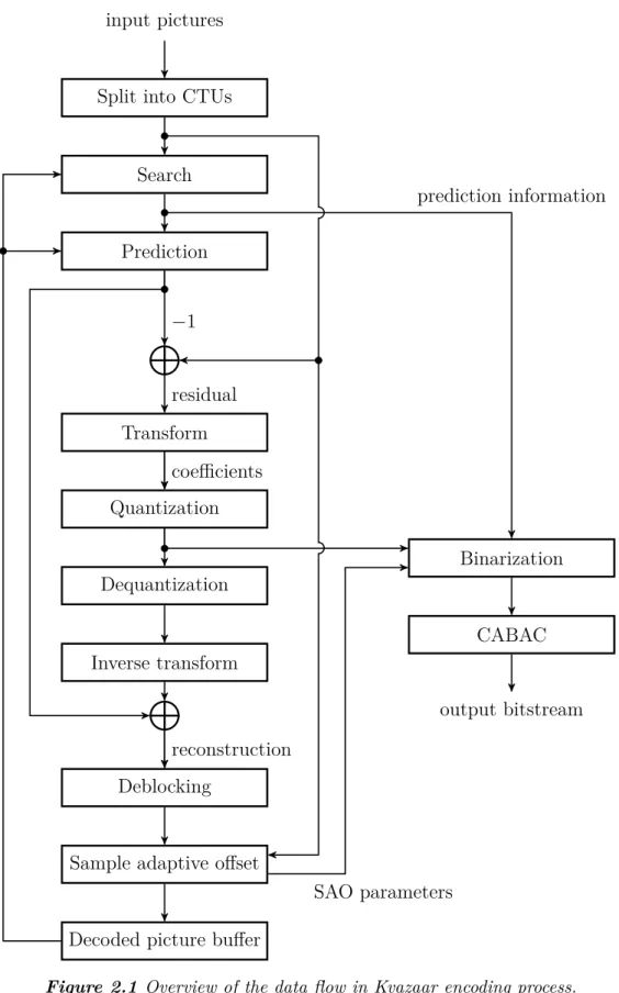
Figure 2.1 depicts the components of Kvazaar and the data flow between them. The input pictures are first split into 64×64 pixel blocks calledcoding tree units(CTUs), which are then processed separately. The phases of the coding process are roughly the same for each CTU. First, the search module attempts to find a way to code the CTU with the lowest coding cost. The inputs to the search are the input picture and the previously coded reference pictures from the decoded picture buffer. The search outputs the prediction information, which specifies how to split the CTU into coding units (CUs) and what is the prediction mode used for each CU.

Next, the prediction module uses the prediction information to construct a prediction for the CTU. The idea is to use previously coded pixels in the current picture and previous pictures to produce a block of pixels that match the CTU as closely as possible. The prediction information specifies which pixels are used to generate the prediction. Using pixels from previously coded pictures is referred to asinter-picture predictionor simplyinter prediction, whereas prediction using only information from the current picture is called intra-picture prediction orintra prediction.

The difference between the input picture and the prediction is called the residual. The residual undergoes a transformation into the frequency domain resulting in a matrix of coefficients. The coefficients are then quantized in order to reduce the number of bits needed to represent them. The quantization and transform are subsequently reversed in dequantization and inverse transform. The result of the inverse transform is the residual that will be available on the decoder side. This new residual is added to the original prediction, resulting in the reconstruction of the CTU.

Finally, two in-loop filters,deblocking andsample adaptive offset (SAO), are applied to the reconstruction. The filtered reconstruction is stored in the decoded picture buffer for later use in the inter prediction of subsequent frames.

The pieces of information required for bit stream generation are the prediction infor-mation from search, the quantized coefficients after transform and quantization, and the SAO parameters. The first step is converting the information to syntax elements that follow the HEVC standard. The syntax elements are then passed through bina-rization andcontext-adaptive binary arithmetic coding (CABAC), which is the final,

(16)

2.3. Overview of the coding process 6

input pictures

Split into CTUs

Search Prediction Transform Quantization Dequantization Inverse transform Deblocking

Sample adaptive offset

Decoded picture buffer

Binarization CABAC output bitstream SAO parameters prediction information −1 residual coefficients reconstruction

(17)

2.4. Coding unit structure 7 A B C D E F G H I J K L M N O P Q R S A B CDE F G H I J KLM N OPQR S 64×64 32×32 16×16 8×8

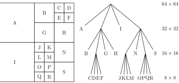
Figure 2.2 An example of a CTU split into CUs and the corresponding quadtree.

lossless compression step. The encoder then outputs the resulting bit stream.

2.4

Coding unit structure

The input video frame is first divided into CTUs according to the HEVC coding structure. The size of a CTU is signaled in the bit stream headers. The HEVC standard permits the sizes of 64×64, 32×32, and 16×16 luma pixels, thus providing the flexibility needed to support various applications [14]. Kvazaar uses only the largest CTU size of 64×64.

A CTU may be coded as a single CU or the encoder may decide to split it into four quadrants. The quadrants may be further divided into smaller quadrants, until the minimum CU size is reached. The minimum CU size is also signaled in the bit stream headers and it must be between 8×8 luma pixels and the selected CTU size. Kvazaar supports a complete HEVC coding tree down to the size of 8×8 pixels. The structure of the CU tree is determined in the search phase. For a homogeneous region, a large CU may be chosen since it requires fewer bits than using multiple smaller CUs [14]. Conversely, an area with small details may be better represented by using several small CUs. An example of a 64×64 CTU split into CUs is given in Figure 2.2.

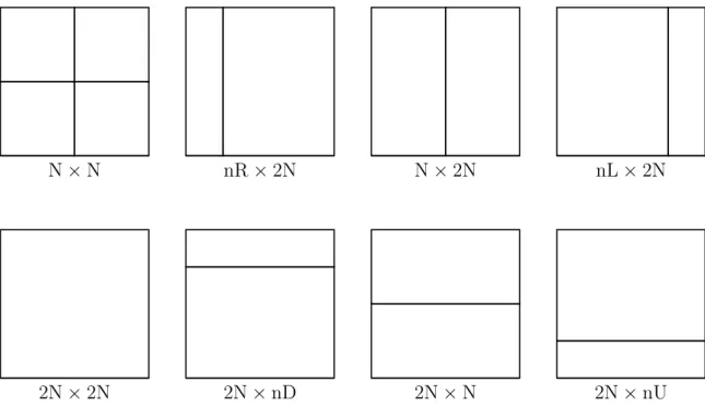
A CU contains one or moreprediction units (PU). A single CU must use either intra or inter prediction, but the prediction parameters may be different in each PU. The partition into PUs is determined by the partition mode of the CU. The possible partition modes are illustrated in Figure 2.3. The N×N partition mode can only be

(18)

2.5. Prediction modes 8

2N×2N 2N×nD 2N×N 2N×nU

N×N nR×2N N×2N nL×2N

Figure 2.3 Partition modes available in HEVC.

used in intra predicted CUs of the minimum size. The non-square partition modes 2N×N, N×2N, 2N×nU, 2N×nD, nL×2N, and nR×2N are only available for inter-predicted CUs. Kvazaar does not consider the non-square partition modes by default, making the 2N×2N mode the one most often used.

In addition to the partition into PUs, each CU is also divided into one or more transform units (TUs) whose size is between 4×4 and 32×32 luma pixels. Each TU is handled separately in the transform and quantization phases. The TUs form a quadtree structure similar to that of the CU quadtree: any unit may be recursively split into four quadrants all the way down to the minimum TU size. However, splitting a CU into multiple TUs only leads to minute gains in coding efficiency [14]. Therefore, Kvazaar always sets the TU size equal to the CU size, except for CUs of size 64×64, which must be split into four TUs of size 32×32 luma pixels.

2.5

Prediction modes

There are two possible prediction modes: intra prediction and inter prediction. Each CU uses one of these two modes. As the names suggest, intra-predicted CUs refer to the pixels within the same picture and inter CUs refer to the pixels in previously coded pictures.

(19)

2.5. Prediction modes 9

left reference

top-left reference top reference

Figure 2.4 Reference pixels for intra prediction.

2.5.1

Intra prediction

Intra PUs are predicted based on the reference pixels obtained from the neighboring blocks. Figure 2.4 shows the pixels used to form the left and top references. If the reference pixels are not available, for example due to the PU being located at the edge of the picture, they are generated by copying the nearest available pixels. The intra mode of a PU determines how the reference pixels are used to predict the pixels within the block. The intra mode can be the DC mode, the planar mode or one of the 33 angular modes. When the DC mode is used, the same value is used for all pixels within the PU. This value is computed as the arithmetic mean of the references pixels.

The angular modes provide a good prediction for directional patterns, such as edges [15]. Each pixel within the PU is predicted by using a linear interpolation between the two nearest reference pixels from the direction specified by the angu-lar mode. The 33 directions are distributed so that the available angles are denser near the vertical and horizontal directions and get sparser towards the diagonal an-gles. This improves the coding efficiency for real-life video, which contains more horizontal and vertical patterns than diagonal patterns [15].

For smooth regions, the angular modes may cause contouring artifacts and the DC mode may lead to blockiness [16]. The planar mode may provide a better prediction in these cases. In the planar mode, the prediction of a pixel is based on the reference pixels located directly above and directly to the left of the pixel, as well as the

(20)

2.5. Prediction modes 10 reference pixels diagonally adjacent to the bottom-left and top-right corners of the block. The value of the pixel is the average of two linear interpolations. The planar prediction is continuous at the edges of blocks and therefore avoids the artifacts that may appear when using DC or angular modes [16].

2.5.2

Inter prediction

The prediction parameters for inter predictive PUs are the number of the picture that is used as the reference and a motion vector (MV). The MV is added to the coordinates of the PU and the resulting coordinates in the reference frame are used as the origin of the prediction. An area matching the size of the PU is then copied from the reference frame to the current frame.

The process where the encoder determines the best MV is known asmotion estima-tion (ME). Since the number of possible MVs is prohibitively large, typically only a subset of them is evaluated. The algorithms for choosing which MVs are checked are known as a block matching algorithms (BMA). Kvazaar has support for three BMAs: 1) hexagon-based search (HEXBS) [17]; 2) test zone search, which is also used by HM [7]; and 3) full search.

The MVs are given at a quarter-pixel precision, which means that it is possible to point to fractional coordinates. This is referred to as fractional motion estimation (FME). The pixel values at fractional coordinates are interpolated from the sur-rounding pixels using a 4-tap, 7-tap or 8-tap filter [18]. The filtering process is slow due to the large number of memory accesses and arithmetic operations required, but the use of fractional MVs can greatly improve the coding efficiency [18].

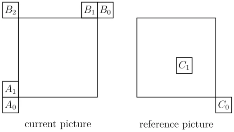
The MV is transmitted to the decoder as a difference to a motion vector predictor (MVP). The MVP candidates are generated for each inter PU in a process known as advanced motion vector prediction (AMVP). Five spatial MVP candidate positions and twotemporal motion vector prediction (TMVP) candidate positions are used in AMVP. The locations of the spatial and temporal candidate positions are illustrated in Figure 2.5. The spatial MVP candidates are located on the left and top sides of the current PU because the blocks to the right and below in the current picture will be encoded later. The motion information from the right and bottom can be harnessed by choosing the temporalC0 candidate [19].

Two MVP candidates are then chosen among the candidate positions according to their availability. A candidate position is deemed unavailable if the PU at the candidate position is outside the picture frame, uses intra prediction, or has not

(21)

2.6. Transform and quantization 11 A0 A1 B0 B1 B2 current picture C0 C1 reference picture

Figure 2.5 Locations of the spatial and temporal AMVP candidates.

been coded yet. The encoder writes the index of the candidate used as the MVP, and the difference between the MVP and the actual MV to the bit stream.

The HEVC standard also supportsbi-prediction, that is, prediction from two differ-ent reference frames. In this case, a possibly weighted average of the two predictions is computed. Bi-prediction is implemented in Kvazaar, but is disabled by default. Generally, it is not possible to use a quadtree structure to cleanly divide the picture into regions of similar motion [20]. For example, when only a single quadrant of a block contains differing motion, it must be divided into four blocks even though the other three quadrants will then have redundant motion. The redundancy is a significant issue: blocks that share the motion information of their neighbors make up approximately 40 % of all blocks [21]. The problem can be mitigated by merging similar blocks after the quadtree division [20]. In HEVC, this is achieved by using the merge mode. When a PU is marked as merged, its reference frame index and MV are copied from one of its merge candidates, saving the bits that would have been needed for coding the motion information. There are five merge candidates, which are chosen among the same candidate positions as the AMVP predictors. For inter CUs that use the merge mode and a partition size of 2N×2N, the encoder can use theskip mode. When using the skip mode, the residual coefficients are set to zero and the partition size and prediction mode are implied. They need not be signaled in the bit stream so a few bits can be saved.

2.6

Transform and quantization

After prediction, the residual is computed as the difference between pixel values in the input picture and the prediction. The residual is transformed using either discrete sine transform(DST) for the luma transform of 4×4 TUs, ordiscrete cosine

(22)

2.7. In-loop filters 12 transform (DCT) for all other TUs. The transforms compute the coefficients for the frequency components present in the picture data.

Next, the coefficients are quantized. The quantization step has the greatest effect on the trade-off between distortion and bit rate. The number of quantization levels is derived from thequantization parameter (QP), which can be given as an input to the encoder. A higher QP means that fewer quantization levels are used, reducing the number of bits spent but increasing distortion. A lower QP corresponds to more quantization levels. This reduces distortion but costs more bits.

During quantization, the encoder can make small changes to the coefficients in order to control whether they are rounded up or down. These adjustments can reduce the number of bits required for coding the coefficients. Optimizing coding efficiency by changing the coefficients is referred to as rate–distortion optimized quantization (RDOQ). It can give a significant improvement in coding efficiency, but the additional computation required to evaluate the coefficient adjustments will reduce coding speed [22].

Transform and quantization are then reversed, as in the decoding process. First, the quantized coefficients are dequantized. Then the inverse transform is performed on the dequantized coefficients. Finally, the predicted pixels are added, resulting in the unfiltered reconstruction, which is then passed to the in-loop filters.

2.7

In-loop filters

Two filters may be applied to the reconstructed pixels before they are added to the decoded picture buffer. The deblocking filter can counteract the artifacts caused by partitioning the video to rectangular blocks [16]. It is applied only at the edges of PUs and TUs. The SAO filter, on the other hand, is applied to all pixels. It can be used to reduce ringing artifacts near edges or to correct a systematic error in the pixel values of a CTU [16]. Since the filters aim to correct different types of artifacts, it is useful to apply both of them [16].

2.7.1

Deblocking filter

The deblocking filter consists of two parts: horizontal filtering and vertical filtering. Conceptually, horizontal filtering is applied first for all vertical edges in the picture and then vertical filtering is applied for all horizontal edges. In practice, Kvazaar applies both vertical and horizontal filtering to an area as large as possible imme-diately after the reconstruction of a CTU. The rest of the CTU is deblocked as the

(23)

2.7. In-loop filters 13 required information becomes available, that is, when the neighboring CTUs have been reconstructed.

The edges to be filtered are the PU and TU borders whose coordinates are divisible by eight. The filtering affects the nearest 4 luma pixels and 2 chroma pixels in both directions from the edge.

2.7.2

Sample adaptive offset (SAO)

SAO adjusts the samples by adding an offset to the intensities of some of the samples. There are two SAO modes available in HEVC:band offset and edge offset. For each CTU, the encoder decides to use a band offset, an edge offset, or no offset at all. In addition, the encoder must choose the parameters for the SAO mode used. These parameters along with the SAO mode are signaled to the decoder in the bit stream. In the case of band offset, the range of possible pixel values is divided into eight bands of equal size. For example, when the bit depth is eight, each band covers 28_/_{8 = 32} values. The encoder must choose four consecutive bands and offsets for each of them. The four offsets are then added to the values of all pixels whose intensities are within the corresponding band. This can be used to correct a systematic error in sample intensity.

When edge offset is chosen instead, each pixel is classified into one of the five cate-gories. The classification depends on the intensities of the pixel and two neighboring pixels. The neighboring pixels are taken from the opposite sides of the pixel accord-ing to the edge direction chosen by the encoder. There are four possible directions: horizontal, vertical and two diagonal directions.

The categorization for edge offset is defined as follows. Category 0 contains pixels whose intensity is between the intensities of its neighbors. Category 1 contains pixels whose intensity is less than that of its neighbors. Category 2 contains pixels whose intensity is equal to one of its neighbors and less than the other. Category 3 contains pixels whose intensity is equal to one of its neighbors and greater than the other. Category 4 contains pixels whose intensity is greater than that of its neighbors. The encoder then chooses an offset for each of the categories. The offset is added to the values of all pixels in the category. The offset must be zero for category 0, non-negative for categories 1 and 2, and non-positive for categories 3 and 4, thereby smoothing the picture. This kind of smoothing can reduce ringing artifacts where an echo appears near edges [16].

(24)

2.8. Entropy coding 14

2.8

Entropy coding

The final phase of the encoding process is the generation of the actual bit stream. The bit stream is formed based on the prediction information, quantized coefficients, and SAO parameters. In addition, the headers of each coded picture and the whole sequence are filled with some general data, for example, the dimensions of a picture and a list of enabled coding tools.

All information that is to be transmitted to the decoder is first mapped into HEVC syntax elements. The syntax elements of the headers are output directly, but most of the other elements are further compressed with CABAC. These syntax elements are converted into a sequence of binary symbols (bins) in the binarization step. Each bin is associated with a context, which is generally determined by the type of syntax element it represents, but may also depend on side information, such as the size of the related CU, PU or TU.

The CABAC module models the distribution of bins for each context. It can there-fore accurately estimate the probability of each bin [23]. The probability models are continuously updated as more bins are coded so they can adapt to variations in the bin distribution [16]. The arithmetic coder can then take advantage of the probabilities to encode the bins losslessly while using fewer bits than the number of bins.

2.9

Parallelization

There are two main approaches to parallel HEVC encoding and decoding: tiles and wavefront parallel processing (WPP). In both approaches, the picture to be coded is divided into parts that can be encoded in parallel. Kvazaar supports both tiles and WPP.

In addition to parallelism within a single picture, picture-level parallel processing is also possible. When a frame either uses intra prediction only or has all of its reference frames already encoded, its encoding can be started without waiting for other frames to be completed.

2.9.1

Tiles

When tiles are used for parallelism, the video is divided horizontally and vertically along CTU boundaries into a number of tile rows and tile columns. The result is a

(25)

2.10. Kvazaar options 15 partition of the video into rectangular areas called tiles. The dependencies between CTUs belonging to different tiles are removed by disabling MV merge and intra prediction across tiles as well as resetting the CABAC states at the start of every tile [24]. Each tile of a single picture can therefore be encoded independently, allow-ing parallel encodallow-ing. However, due to removed dependencies, the codallow-ing efficiency suffers greatly [24].

2.9.2

Wavefront parallel processing (WPP)

WPP allows processing CTU rows in parallel. However, the rows are not made completely independent. After the second CTU of a row is completed, the CABAC probabilities are copied to be used for coding the first CTU of the row below. There-fore, the encoding of each CTU must wait until the row above has advanced two CTUs further than the current row. The loss of coding efficiency remains small be-cause intra prediction and MV merge need not be limited and CABAC probabilities are propagated [24].

Instead of dedicating a specific thread for each CTU row, Kvazaar lets any thread choose any available CTU as its next piece of work [25]. This helps in minimizing thread idle time. For example, if a CTU row is stalled because a CTU in the row above is taking longer than expected, the thread that was working on that row can start working on a CTU in some other frame instead of waiting.

WPP can further improve picture-level parallelism by using overlapped wavefronts (OWF), which allow an inter frame and its reference frames to be encoded in parallel. The processing of the next frame is started after only a few CTU rows in the current frame have been completed [24]. This requires that the maximum length of MVs is restricted so that they cannot point to the parts of the previous frame that have not been coded yet.

2.10

Kvazaar options

Kvazaar provides several options that can be used to turn coding tools on and off. For ease of use, ten sets of preferred options, called presets, have been devised. Each preset gives a different trade-off of coding efficiency for speed. The presets are ultrafast, superfast, veryfast, faster, fast, medium, slow, slower, veryslow, and placebo, in the order of increasing complexity and coding efficiency. The placebo preset turns on all options for maximum coding efficiency without any regard for

(26)

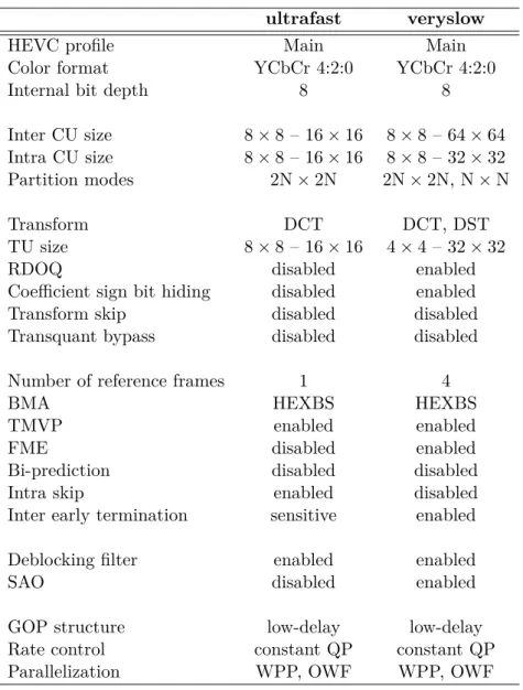
2.10. Kvazaar options 16 Table 2.1 Kvazaar coding tools with the analyzed presets.

ultrafast veryslow

HEVC profile Main Main

Color format YCbCr 4:2:0 YCbCr 4:2:0

Internal bit depth 8 8

Inter CU size 8×8 – 16×16 8×8 – 64×64 Intra CU size 8×8 – 16×16 8×8 – 32×32 Partition modes 2N×2N 2N×2N, N×N

Transform DCT DCT, DST

TU size 8×8 – 16×16 4×4 – 32×32

RDOQ disabled enabled

Coefficient sign bit hiding disabled enabled Transform skip disabled disabled Transquant bypass disabled disabled Number of reference frames 1 4

BMA HEXBS HEXBS

TMVP enabled enabled

FME disabled enabled

Bi-prediction disabled disabled

Intra skip enabled disabled

Inter early termination sensitive enabled Deblocking filter enabled enabled

SAO disabled enabled

GOP structure low-delay low-delay Rate control constant QP constant QP Parallelization WPP, OWF WPP, OWF

complexity. It is much slower than the veryslow preset, but achieves only slightly better coding efficiency. Therefore, we will exclude it from our analysis.

We choose to focus on the two practical presets that represent the two extremes of the complexity–efficiency trade-off: ultrafastandveryslow. Table 2.1 lists the coding tools of Kvazaar with these presets. The ultrafast preset seeks the fastest possible encoding speed so only the very basic coding tools are enabled.

Compared with theultrafast preset, theveryslow preset enables most of the remain-ing codremain-ing tools and disables the optimizations that sacrifice codremain-ing efficiency for speed. CUs of size 32×32 are enabled for both intra and inter prediction. The largest CUs of size 64×64 are only used for inter. Intra prediction, on the other hand, can take advantage of the smallest 4×4 prediction units through the use of the N×N partition mode. In addition, the number of reference frames is quadrupled.

(27)

2.10. Kvazaar options 17 With all preset levels, the trade-off between the distortion and size of the compressed bit stream can be controlled by setting either the QP or the target bit rate. When the target bit rate is set, Kvazaar will attempt to adjust the QP for each CTU so that the average bit rate matches the target.

Kvazaar uses aλ domain rate control algorithm with hierarchical bit allocation [26]. First, the video sequence is divided into short segments called groups of pictures (GOPs), which are typically four to eight pictures long. The target number of bits per GOP is set based on the number of pictures and bits coded in the past so that the target bit rate is met over time. Next, the bit budget for the GOP is divided among the pictures. This allocation is based on a GOP structure, which defines a weight for each picture in the GOP. Pictures that are not used as a reference are usually given a lower weight. The GOP structure in Kvazaar is static, meaning that the same weights are used for each GOP. Finally, the size of the picture header is subtracted from the bit budget of the picture and the rest is divided among the CTUs of the picture. CTUs are weighted based on the distortion of the co-located CTU in the previous picture [26]. A CTU with high distortion is given more bits in the next picture so that the distortion can be reduced.

Kvazaar seeks to meet the bit rate target for a CTU by adjusting the Lagrange multiplierλ. The bit rate and λ are assumed to satisfy

λ=αRβ_bpp, (2.1)

where Rbpp is the bit rate in number of bits per pixel [26]. The values of α and β are dependent on the video content and are updated after each encoded CTU [26]. The value of λset according to Equation (2.1) is then used to derive the QP value. If no bit rate target is set, Kvazaar uses a constant QP. This results in a consistent quality, but may cause fluctuations in bit rate. Rate control is not the focus of this work so we use a constant QP.

(28)

18

3.

METHODOLOGY

In video coding, there are three quantities of interest: bit rate, quality, and complex-ity. Bit rate is the number of bits that the encoder spends on encoding a sequence of pictures. Quality measures the similarity of compressed video and the original one. A high quality means that there is little to no distortion in the compressed video. Here, complexity refers to the amount of time spent by the encoder.

The bit rate and quality can be incorporated into a single value called the coding efficiency. Reducing bit rate or improving quality leads to higher efficiency. Im-provements in complexity often come with a trade-off in coding efficiency and vice versa.

This section defines the methods used for measuring the improvements in coding efficiency and complexity.

3.1

Coding efficiency

Computation of coding efficiency requires that we first measure the bit rate and distortion. It is easy to measure the bit rate by counting the number of bits the encoder outputs. For distortion, a comparison with the original video sequence is necessary. The distortion is measured as the peak signal-to-noise ratio (PSNR) which is defined in terms of the mean squared error (MSE). Given a monochrome reference imageI and a compressed image ˆI of size W ×H pixels, the MSE is

MSE = 1 W ·H H ∑ i=1 W ∑ j=1 ( Iij −Iˆij )2 .

When computing the PSNR for a sequence with bit depthB, we compare the MSE with the maximum value 2B₋_{1 of a single pixel. All the test sequences we use have}

bit depth of B = 8. The PSNR is then

PSNR = 10·log₁₀ (

2B₋₁)2

(29)

3.2. Complexity 19 PSNR is measured using a logarithmic scale. As MSE approaches zero, PSNR approaches infinity. Accordingly, a higher PSNR corresponds to less distortion and higher quality.

All video sequences in our tests are in color. Therefore, the PSNR must be measured separately for the luma (PSNRY) and chroma (PSNRCb and PSNRCr) components. The combined PSNR is a weighted average of the component PSNR values [27]:

PSNRYCbCr =

6·PSNRY+ PSNRCb+ PSNRCr

8 .

The average PSNR of a video sequence is the arithmetic mean of the PSNRYCbCr values for each frame of the sequence [27]. If the encoder manages to encode a frame with zero distortion, the PSNR for that frame, as well as the average PSNR for the sequence, would be infinite. In practice, however, with the used test sequences, there is always some distortion so this does not pose a problem.

The coding efficiency of two encoders can be compared by combining the bit rate and distortion into a single quantity, theBjøntegaard-delta bit rate (BD-rate) [28]. BD-rate is calculated as follows. First, the test sequences are encoded with four different QP values using both the tested encoder and the anchor. The HEVC common test conditions [29] specify the QP values of 22, 27, 32, and 37, which are also used in this work. Bit rate and distortion are then measured for each of the coded sequences in these four operating points. The bit rate is converted to a logarithmic scale because a linear scale would overly emphasize high bit rates [28]. Next, a third-order polynomial curve is fitted so that it passes through the four rate– distortion points [28]. The area under each curve is then calculated by integrating over the longest interval where both curves are defined [28]. Finally, the BD-rate is the difference between the areas under the two curves.

A negative BD-rate can be interpreted as meaning that, in order to achieve the same quality, the tested encoder needs fewer bits than the anchor does. Conversely, a positive BD-rate means that the encoder spends more bits than the anchor.

3.2

Complexity

We measure encoder complexity by running the encoder multiple times and taking the arithmetic mean of the running times. In order to prevent interference from other programs, all other applications are closed and only one test is run at a time. The first run with a given encoder and test sequence is discarded because it is typically considerably slower since the operating system has not cached the encoder binary

(30)

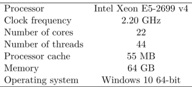
3.3. Test material 20 Table 3.1 Properties of the test computer.

Processor Intel Xeon E5-2699 v4 Clock frequency 2.20 GHz Number of cores 22 Number of threads 44 Processor cache 55 MB

Memory 64 GB

Operating system Windows 10 64-bit

and the video file yet.

The value of the QP not only determines the video quality, but indirectly affects the encoding speed too. With low QP values, more symbols are used to encode the residual coefficients. The coefficient symbols are compressed using the slow CABAC process so encoding a sequence using a low QP takes more time than encoding it with a higher QP.

In our measurements, we encode each test sequence twice with each of the same four QP values that are used in coding efficiency tests: 22, 27, 32, and 37. For each QP, we average the two running times and compare the average time with the anchor. The speedup of the tested encoder is the ratio of the time taken by the anchor and the time taken by the tested version of the encoder. Finally, the average speedup for a given video sequence is the arithmetic mean of the speedups with the four tested QP values.

All complexity measurements are run on a 22-core Intel Xeon E5-2699 v4 processor. The details of the computer are listed in Table 3.1.

3.3

Test material

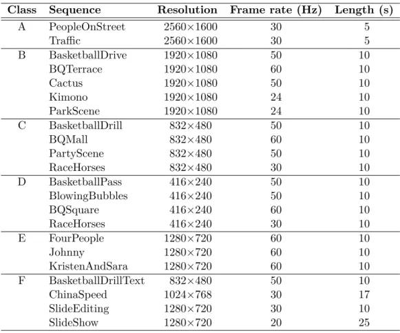
The HEVC common test conditions [29] define a set of 24 test sequences of different size and content. For our tests, we use the 22 sequences that have a bit depth of 8. These sequences are listed in Table 3.2. The sequences are divided into classes from A to F. Sequences in classes A, B, C, and D contain varied content of sizes 2560×1600, 1920×1080, 832×480 and 416×240, respectively. Class E is composed of video conferencing content of size 1280×720 with a stationary camera. Class F contains screen content, such as computer-generated graphics, of various sizes. Most sequences are 10 seconds long, but there are a few shorter and longer ones as well.

(31)

3.3. Test material 21

Table 3.2 Details of the test sequences.

Class Sequence Resolution Frame rate (Hz) Length (s)

A PeopleOnStreet 2560×1600 30 5 Traffic 2560×1600 30 5 B BasketballDrive 1920×1080 50 10 BQTerrace 1920×1080 60 10 Cactus 1920×1080 50 10 Kimono 1920×1080 24 10 ParkScene 1920×1080 24 10 C BasketballDrill 832×480 50 10 BQMall 832×480 60 10 PartyScene 832×480 50 10 RaceHorses 832×480 30 10 D BasketballPass 416×240 50 10 BlowingBubbles 416×240 50 10 BQSquare 416×240 60 10 RaceHorses 416×240 30 10 E FourPeople 1280×720 60 10 Johnny 1280×720 60 10 KristenAndSara 1280×720 60 10 F BasketballDrillText 832×480 50 10 ChinaSpeed 1024×768 30 17 SlideEditing 1280×720 30 10 SlideShow 1280×720 20 25

(32)

22

4.

PROPOSED OPTIMIZATIONS

We implemented four main optimizations to Kvazaar:

Optimization 1. Uniform inter and intra cost comparison Optimization 2. Concurrency-oriented SAO implementation Optimization 3. Resolution-adaptive thread allocation Optimization 4. Fast cost estimation of coding coefficients

In this chapter, these changes are described on the technical level and their indi-vidual impact on performance is analyzed. The overall effects of the changes and a comparison to other open-source HEVC encoders are presented in Chapter 5.

4.1

Uniform inter and intra cost comparison

In all-intra coding, Kvazaar was already on par with the other open-source HEVC encoders [30], particularly the most well known encoder, x265 [10]. However, in inter coding, Kvazaar was still behind x265 in both coding efficiency and complexity. Since Kvazaar was performing well in all-intra coding, it seemed plausible that there room for optimization either in inter motion estimation or in the process of deciding whether to use intra or inter prediction.

No immediate opportunities for optimization were found in motion estimation so we decided to look for possible optimizations in the prediction mode decision. As the first step, we analyzed how large portions of the video were coded using intra prediction and inter prediction. We wanted to focus the analysis on the prediction mode decision process and, therefore, wanted to limit the number of coding tools to the absolute minimum in order to remove the possibility of defects in Kvazaar coding tools causing interference. Hence, theultrafast preset was used for both encoders. Next, we modified the decoder part of the HM software [7] to print the prediction mode and size for each decoded CU. All test sequences were then encoded with both

(33)

4.1. Uniform inter and intra cost comparison 23 Table 4.1 Kvazaar CU size and mode usage.

Size Inter (%) Intra (%) Total (%)

8×8 79.28 0.32 79.60

16×16 20.29 0.10 20.39

32×32 0.00 0.01 0.01

Total 99.57 0.43 100.00

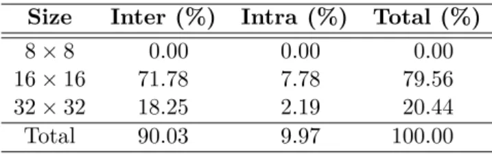
Table 4.2 x265 CU size and mode usage.

Size Inter (%) Intra (%) Total (%)

8×8 0.00 0.00 0.00

16×16 71.78 7.78 79.56 32×32 18.25 2.19 20.44 Total 90.03 9.97 100.00

Kvazaar and x265 and the generated bit streams were decoded using this modified decoder. Finally, a Python script was used to read the results and compute the percentages of each CU size and prediction mode. These are tabulated in Table 4.1 and Table 4.2.

According to the results, x265 coded 10 % of the CUs with intra prediction, whereas Kvazaar used intra prediction for fewer than 1 % of the CUs. This was an interesting discovery, since it was intra coding where Kvazaar surpassed x265. One possible explanation for the low percentage of intra prediction was the intra skip mechanism, which Kvazaar employed with the fastest presets. The essence of the intra skip is that when the best MV found in inter motion estimation is deemed good enough (distortion and cost in bits are below a predefined threshold), the search for a suitable intra prediction mode is skipped altogether. This yields a considerable speedup at the expense of BD-rate.

We ran the tests again with intra skip turned off. The new percentages are shown in Table 4.3. Disabling intra skip raised the use of intra prediction in Kvazaar to 4 % of the CUs, which was better than before but still far from the 10 % used by x265.

Table 4.3 Kvazaar CU size and mode usage with intra skip disabled.

Size Inter (%) Intra (%) Total (%)

8×8 77.39 2.86 80.25

16×16 18.87 0.77 19.64

32×32 0.00 0.11 0.11

(34)

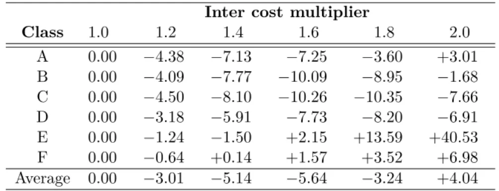
4.1. Uniform inter and intra cost comparison 24 Table 4.4 BD-rate for different inter cost multiplier values.

Inter cost multiplier

Class 1.0 1.2 1.4 1.6 1.8 2.0 A 0.00 −4.38 −7.13 −7.25 −3.60 +3.01 B 0.00 −4.09 −7.77 −10.09 −8.95 −1.68 C 0.00 −4.50 −8.10 −10.26 −10.35 −7.66 D 0.00 −3.18 −5.91 −7.73 −8.20 −6.91 E 0.00 −1.24 −1.50 +2.15 +13.59 +40.53 F 0.00 −0.64 +0.14 +1.57 +3.52 +6.98 Average 0.00 −3.01 −5.14 −5.64 −3.24 +4.04

Guided by these results, we applied a penalty multiplier to the cost of using inter in order to force Kvazaar to use more intra prediction. We tested several values for the multiplier ranging from 1.0 to 2.0. The BD-rate improvements for each multiplier are listed in Table 4.4.

The best average BD-rate improvement was −5.64 %, corresponding to the cost multiplier of 1.6. For many sequences, the decrease in BD-rate was over 10 %, but for a few sequences, it increased instead. This proved that there was indeed a deeper issue in the logic for deciding whether to use intra or inter prediction.

The decision on which intra mode or inter MV to use for a block is based on the notion ofrate–distortion cost(RD-cost), which takes into account both the distortion and the number of bits used for the block. The cost is computed for each of the prediction parameters checked and the one with the lowest cost is chosen.

Like HM, Kvazaar employs three distortion metrics: 1) the sum of squared er-rors (SSE); 2) the sum of absolute differences (SAD); and 3) the sum of absolute Hadamard-transformed differences (SATD). In the case of SSE, the cost of a block is

JSSE = SSE +λ·R,

where rate R is the number of bits spent. Lagrange multiplier λ defines the trade-off between bit rate and distortion. The SSE is the slowest but the most accurate metric since it relates directly to the MSE and PSNR, which we use to measure the visual quality. Due to its complexity, Kvazaar only uses SSE when making the decision on whether to use one large CU or to split it into four smaller ones.

The fastest distortion metric used in Kvazaar is the SAD. Since the value of the SAD is less than that of SSE, using the sameλ would give too much weight for the

(35)

4.1. Uniform inter and intra cost comparison 25 bit rate. Hence, the square root of λ is used, and the SAD cost is

JSAD = SAD + √

λ·R.

The third metric used is the SATD, which is similar to SAD, but the differences undergo a Hadamard transform before we take the absolute value and calculate the sum. As with the SAD cost, the square root ofλ is used. The SATD cost is

JSATD = SATD + √

λ·R.

The Hadamard transform is similar to the DCT so it gives a good approximation of the cost of coding the residual coefficients while also being significantly faster than the DCT.

Kvazaar used SATD to evaluate the intra prediction modes. However, a careful re-view of the code revealed that in inter motion estimation the cost was first computed using SAD and then recalculated using SATD if either FME or bi-prediction was performed. However, when neither FME nor bi-prediction were enabled, the costs computed with SAD were never replaced. Bi-prediction is disabled by default on all presets and FME is disabled for the two fastest presets. Hence, when using one of the two fastest Kvazaar presets, the inter SAD costs were being compared with the intra SATD costs. SATD typically gives a cost several times larger than SAD, which explains the fact that intra prediction was hardly used at all.

Our solution was to use SATD costs in all cases by removing the cost multiplier penalty and adding a step for recalculating the inter costs with SATD before making the comparison to the intra cost. We verified, using the modified version of HM decoder, that Kvazaar now used intra prediction for 30 % of the CUs. The BD-rate decreased by a further 4.96 % over the inter cost multiplier.

The final step was to update the intra skip threshold. Originally, the threshold value was 20, which meant that the intra search was skipped when the SAD cost for the block was less than 20 per pixel. The original threshold was found to reduce coding efficiency too much so we decided to test possible values in the range from 0 to 20. The effects on BD-rate and complexity for each value are tabulated in Table 4.5. We settled on the value of 8 as a good compromise between coding efficiency and complexity at fast presets.

Overall, the fix affected complexity in two ways. First, the added SATD calculation increased the time spent in inter search. Second, the new value selected for intra

(36)

4.1. Uniform inter and intra cost comparison 26

Table 4.5 BD-rate and speedup for different intra skip threshold values.

Intra skip threshold Average BD-rate (%) Average speedup

0 0.00 1.00× 2 −0.39 1.01× 4 −0.37 1.04× 6 +0.91 1.11× 8 +2.67 1.17× 10 +4.68 1.22× 12 +6.98 1.26× 14 +9.14 1.29× 16 +11.14 1.31× 18 +13.04 1.33× 20 +14.81 1.35×

Table 4.6 Effect of Optimization 1 on BD-rate and complexity.

Class Sequence BD-rate (%) Speedup

A PeopleOnStreet −24.18 0.84× Traffic −8.93 0.91× B BasketballDrive −30.76 0.80× BQTerrace −18.81 0.73× Cactus −19.88 0.80× Kimono −12.47 0.85× ParkScene −11.92 0.78× C BasketballDrill −25.73 0.84× BQMall −17.28 0.80× PartyScene −14.07 0.75× RaceHorses −23.96 0.80× D BasketballPass −23.47 0.86× BlowingBubbles −10.10 0.77× BQSquare −6.73 0.75× RaceHorses −21.86 0.86× E FourPeople −6.89 0.81× Johnny −3.37 0.97× KristenAndSara −4.92 0.77× F BasketballDrillText −21.04 0.81× ChinaSpeed −15.20 0.88× SlideEditing −2.40 0.74× SlideShow −9.16 0.83× Average −15.14 0.81×

(37)

4.2. Concurrency-oriented SAO implementation 27 skip threshold was less aggressive than the old value. This meant that Kvazaar was not as eager to use the intra skip mechanism so the time spent on intra search was increased as well. Together, these added up to a 20 % slowdown, which was considered a reasonable trade-off for the 15 % lower BD-rate. The effects on coding efficiency and complexity for each test sequence are tabulated in Table 4.6.

4.2

Concurrency-oriented SAO implementation

In order to improve the multi-thread behavior of Kvazaar, we modified Kvazaar to record timing information on the coding process. The collected times were 1) the time when an input frame was read in; 2) the time when Kvazaar started coding a CTU; 3) the time when Kvazaar finished coding a CTU; 4) the time when Kvazaar started generating the bit stream for a frame; and 5) the time when the bit stream generation was finished. The times recorded for a frame were written out to a file after finishing coding the frame.

A separate program was written to visualize the collected data. The visualization, shown in Figure 4.1, displays the state of every CTU at a given point in time. Each square represents a single CTU and the color of the square indicates its state. Gray squares are waiting to be processed, red ones are being coded, and black ones have been completed. The progression of the encoding process can be visualized by moving forward and backwards in time. The upper-left corner displays the time from the start of the encoding in milliseconds. In Figure 4.1, there are six CTUs belonging to three different frames being encoded.

The visualization revealed that when WPP and OWF were enabled, Kvazaar was waiting very long before starting to encode a new frame. The first CTU of the next frame was not started until the last CTU of the second row in the current frame was finished even though not all threads were in use. This was true for other CTU rows too: the inter-frame CTU dependencies were being set up so that the first CTU of any row in a frame always depended on the last CTU of the row below in the previous frame.

The purpose of the inter-frame CTU dependencies is to make sure that the pixels in the reference frame are available when they are used for inter prediction in the current frame. In practice, it is very rare for an inter prediction unit to refer to pixels that are further away than the width of a CTU. Hence, it should be sufficient for a CTU to depend only on the eight CTUs in the reference frame that surround it. Thus, it seemed like Kvazaar was adding unnecessary dependencies.

(38)

4.2. Concurrency-oriented SAO implementation 28

Figure 4.1 Visualization of parallel encoding of a 1280×720 sequence. Each square represents a single CTU. Black squares have been completed, red squares are being coded, and gray squares are waiting to be processed.

The reason for the dependencies was found in the implementation of the SAO filter. Kvazaar applied SAO for a whole CTU row at a time. As a result, when SAO was enabled, it was necessary to wait for the whole row to be completed instead of just a few CTUs in the row. However, these dependencies were being added even when SAO was disabled.

We modified Kvazaar so that when SAO was disabled, the unnecessary inter-frame CTU dependencies were removed, as shown in Figure 4.2. The only inter-frame dependency for each CTU was now the CTU to the right and down of it so it was no longer necessary to wait until the whole row was completed. The intra-frame dependencies guarantee that the eight surrounding CTUs in the reference frame are completed before the processing of the CTU is started. The inter MVs were originally restricted so that they could point to the CTU below but not any further downwards. We added a further restriction to constrain the MVs to the CTUs that were known to be completed at the time. These are shown shaded in Figure 4.2. If the coordinates of the current CTU are (x, y), then the CTUs that can be used for

(39)

4.2. Concurrency-oriented SAO implementation 29 0,0 1,0 2,0 3,0 4,0 0,1 1,1 2,1 3,1 4,1 0,2 1,2 2,2 3,2 4,2 0,3 1,3 2,3 3,3 4,3 0,0 1,0 2,0 3,0 4,0 0,1 1,1 2,1 3,1 4,1 0,2 1,2 2,2 3,2 4,2 0,3 1,3 2,3 3,3 4,3

Figure 4.2 Direct and indirect intra-frame and inter-frame dependencies for a single CTU. The shaded CTUs must be completed before the processing of the CTU (1,1)in the second frame can be started. Redundant indirect dependencies are not shown.

inter prediction, are the CTUs whose coordinates (xi, yi) satisfy

yi ≤y+ 1 ∧ xi+yi ≤x+y+ 2.

Removing the dependencies allowed Kvazaar to exploit the large number of processor cores on the test machine more effectively. We obtained a 2.1×average speedup over all test sequences with the ultrafast preset, which disables SAO. This confirmed that it would be worthwhile to try to change the SAO implementation so that the dependencies could be relaxed even when SAO was turned on. SAO would need to be applied to each CTU as soon as possible. The HEVC specification states that conceptually the deblocking filter is first applied to the whole picture and after that, the SAO filter is applied. Thus, the deblocking filter is the limiting factor in determining when SAO can be applied.

In the Kvazaar deblocking implementation, the right and bottom edges of a CTU are not filtered until the neighboring CTUs to the right and down, respectively, have been reconstructed. This is necessary because pixels on both sides of an edge are required for deblocking. The rightmost 4 luma and chroma pixels of the horizontal edges are also delayed because the right edge of the CTU must be filtered before them. For chroma, it would be sufficient to delay the rightmost 2 pixels, but in order to simplify the implementation, the delay is set to 4 pixels for both luma and chroma. In addition, the right edge of the CTU below must be filtered before the rightmost 4 pixels of the bottom edge of the CTU. The 4×4 pixel block in the bottom-right corner of a CTU is therefore filtered only after the reconstruction of the CTU diagonally to the right and down.

(40)

4.2. Concurrency-oriented SAO implementation 30 56 px 8 px 60 px 4 px (a)Deblocking 54 px 10 px 54 px 10 px (b) SAO

Figure 4.3 CTU split into four regions for in-loop filters.

the rightmost 4 chroma pixels, which cover an area 8 luma pixels wide. As shown in Figure 4.3a, a CTU can be divided into four segments based on when both luma and chroma pixels are fully deblocked: 1) The top-left 56×60 area is deblocked immediately after the reconstruction. 2) The top-right 8× 60 area is deblocked after the reconstruction of the CTU to the right. 3) The bottom-left 56×4 area is deblocked after the reconstruction of the CTU below. 4) The bottom-right 8×4 area is deblocked after the reconstruction of the CTU diagonally to the right and down. If the CTU is located at the edge of the picture so that the adjacent CTUs do not exist, the corresponding areas are deblocked at the same time with the top-left area.

Since computing SAO for a single pixel may require information from the pixels around that pixel, SAO had to be delayed for at least 9 luma pixels at the right edge of the CTU and 5 pixels at the bottom edge. Using odd dimensions would make the code more complex when processing chroma so we decided to round up the values to even numbers. For simplicity, we chose to make the width of the delayed area equal at the bottom and the right side of the CTU, thereby settling on the value of 10 luma pixels.

Figure 4.3b shows how every CTU is divided into four segments for SAO, similarly to the deblocking regions: 1) The top-left 54×54 area is filtered immediately after deblocking. 2) The top-right 10×54 area is filtered after deblocking the CTU to the right. 3) The bottom-left 54×10 area is filtered after deblocking the CTU below. 4) The bottom-right 10×10 area is filtered after deblocking the CTU diagonally to the right and down.

(41)

4.2. Concurrency-oriented SAO implementation 31 Table 4.7 Effect of Optimization 2 on BD-rate and complexity.

ultrafast veryslow

Class Sequence BD-rate (%) Speedup BD-rate (%) Speedup

A PeopleOnStreet 0.00 1.01× −0.03 1.12× Traffic 0.00 0.98× +0.05 1.08× B BasketballDrive 0.00 1.40× +0.02 1.51× BQTerrace 0.00 1.41× 0.00 1.26× Cactus 0.00 1.16× 0.00 1.28× Kimono 0.00 1.29× +0.09 1.28× ParkScene 0.00 1.24× −0.01 1.21× C BasketballDrill 0.00 2.20× −0.03 2.50× BQMall 0.00 2.69× +0.02 2.57× PartyScene 0.00 2.99× +0.01 2.25× RaceHorses 0.00 2.73× −0.05 2.55× D BasketballPass 0.00 1.76× +0.01 1.90× BlowingBubbles 0.00 1.98× 0.00 1.87× BQSquare 0.00 2.08× 0.00 1.86× RaceHorses 0.00 1.86× 0.00 1.92× E FourPeople 0.00 3.45× +0.01 4.34× Johnny 0.00 2.53× 0.00 3.79× KristenAndSara 0.00 2.80× 0.00 4.14× F BasketballDrillText 0.00 2.20× −0.02 2.43× ChinaSpeed +0.01 3.32× −0.01 3.94× SlideEditing +0.20 2.03× +0.33 3.26× SlideShow +0.61 2.68× +2.72 3.89× Average +0.04 2.08× +0.14 2.36×

This change required some changes to Kvazaar data structures. In order to have the information required by SAO available, Kvazaar had to store the pixels that have passed through deblocking but not through SAO. These pixels were originally only stored for the bottommost row of pixels in every CTU. After the change, this storage was changed to store the 54th pixel row, which is overwritten when filtering top-left and top-right parts of the CTU, but is needed when filtering the bottom-left and bottom-right parts. Similar storage was added for the 54th pixel columns of every CTU as well.

SAO filter functions were rewritten so that they could filter any of the four parts to which SAO was applied in a CTU. The decision of the SAO mode and parameters was left as is. Consequently, the SAO parameters would be partly based on the pixels at the bottom and the right side of the CTU that were not yet deblocked. The chosen SAO parameters would therefore be slightly inaccurate, causing a small increase in BD-rate.

(42)

en-4.3. Resolution-adaptive thread allocation 32 abled. The BD-rate and speedup were measured with the ultrafast and veryslow presets. The results are tabulated in Table 4.7. The speedup was even higher with theveryslow preset than with the ultrafast preset. The added potential for picture-level parallelism had the largest effect on the medium-sized sequences, where the number of threads was severely limited by the dependencies. For the high-resolution sequences of classes A and B, the number of threads that fit into a single frame is higher, so most of the available threads were already in use before the change. Con-versely, for the low-resolution sequences of classes C and D, the number of threads in a single frame remained small even after the optimization. The speedup was therefore the highest in class E, where the average speedup was over 4× with the veryslow preset. The BD-rate increased slightly due to the additional restriction on MVs and the SAO parameter selection being based on partly non-deblocked pixels. The loss of coding efficiency was, however, negligible compared with the complexity improvement.

4.3

Resolution-adaptive thread allocation

Discovering the optimization potential in the SAO implementation suggested a fur-ther analysis of the multi-thread behavior of Kvazaar. We measured the speedup with the ultrafast preset in several configurations, varying the video resolutio