www.elsevier.com / locate / econbase
Hybrid models of the Lorenz curve
a ,
*
bTomson Ogwang
, U.L. Gouranga Rao
a
Economics Programme, University of Northern British Columbia, 3333 University Way, Prince George,
British Columbia, Canada V2N 4Z9 b
Department of Economics, Dalhousie University, Halifax, Nova Scotia, Canada B3H 3J5
Received 28 May 1998; accepted 22 December 1999
Abstract
In this paper hybrid Lorenz curves are proposed as a way of circumventing an important drawback of traditional models of the Lorenz curve, namely lack of satisfactory fit over the entire range of a given income distribution. Two categories of hybrid models are identified, namely the additive models and the multiplicative models. Whereas the additive models are obtained by taking convex combinations of the traditional models, the multiplicative models are obtained by taking their weighted products. A comparison of the performances of the hybrid Lorenz curves with those of the constituent Lorenz curves shows that both the additive and multiplicative models perform generally better than the constituent Lorenz curves. 2000 Elsevier Science S.A. All rights reserved.
Keywords: Additive model; Multiplicative model; Hybrid Lorenz curve; Gini index
JEL classification: C80; D30
1. Introduction
The Lorenz Curve (LC), which plots the cumulative share of total income (the ordinate) against the cumulative proportion of income-receiving units (the abscissa), is a powerful graphical device for analyzing the size distribution of income and wealth. The curve is also used to estimate the Gini index and other measures of inequality and poverty.
A number of parametric models that satisfy the basic properties of a LC have been proposed in the literature. See, for example, Kakwani and Podder (1973, 1976), Rasche et al. (1980), Gupta (1984),
˜
Rossi (1985), Arnold (1986), Rao and Tam (1987), Villasenor and Arnold (1989), Basmann et al. (1990), Ortega et al. (1991), Chotikapanich (1993), Schader and Schmid (1994), Ryu and Slottje
*Corresponding author. Tel.: 11-250-960-6485; fax:11-250-960-5544.
E-mail address: [email protected] (T. Ogwang).
(1996), Ogwang and Rao (1996), and Sarabia (1997). Recent research (e.g. Rossi, 1985; Basmann et al., 1990; Ryu and Slottje, 1996) has brought to light the fact that certain models of the LC fit certain segments of the observed income distribution better than others. For example, it is not uncommon for a particular model of the LC to fit, say, the first decile of the observed income distribution better but do poorly when fitted to, say, the ninth decile. In view of this problem, it seems reasonable to construct hybrid LCs by combining two or more traditional models of the LC that fit different portions of the observed income distribution well. As will be seen below, such models are obtained either by taking convex combinations of traditional models of the LC (the additive model) or by taking their weighted products (the multiplicative model). A further advantage of hybrid models of the LC is that they have greater flexibility than the constituent models owing to the inclusion of weighting parameters which must also be estimated. The parameters of hybrid LCs, like those of the constituent LCs, can be consistently estimated by nonlinear least squares (NLS).
The format of the rest of the paper is as follows: Section 2 introduces the two types of hybrid models of the LC and provides expressions for the associated Gini indices. A comparison of the performances of the two hybrid LCs with those of the constituent LCs is made in Section 3. The concluding remarks are made in Section 4.
2. Hybrid models of the Lorenz curve
A LC is defined by the ordered points ( p, y) where p is the cumulative proportion of the income-receiving units and y is the cumulative share of incomes, if the incomes are arranged in ascending order of magnitude. If y5f( p) is a twice-differentiable function defined in the closed interval (0,1), then y describes a LC if and only if the following four properties are satisfied: f(0)50;
2 2
f(1)51; dy / dp$0 for 0#p#1; and d y / dp $0 for 0#p#1. The properties f(0)50 and f(1)51
2 2
ensure that the LC passes through the points (0,0) and (1,1). The properties dy / dp$0 and d y / dp $0 ensure that the LC has the right curvature, i.e. it should be monotonically increasing and convex towards the p-axis with 0#f( p)#p#1.
where 0#d#1, as the additive model of the LC. Estimation of the additive model entails estimation of the parameters of the two constituent LCs and the weighting parameterd.
g l
If y15f ( p) and y1 25f ( p) describe a LC, then their weighted product y2 5f( p)5f ( p) f ( p)1 2 describes a LC certainly when g$1 and l$ 1 but also for other positive values of g and l
g l
depending on the properties of the f ( p)s. To see this, we note that f(0)i 5f (0) f (0)1 2 50; f(1)5
g l g l21 l g21 2 2
f (1) f (1)1 2 51; dy / dp5lf ( p) f ( p)1 2 df ( p) / dp2 1gf ( p) f ( p)2 1 df ( p) / dp1 $0; and d y / dp 5
1
g l21 2 2 l g21 2 2 g21 l21 the two LCs satisfies all the four properties of a LC. For other values of g and l, it is also possible
2 2 2
that d y / dp $0 depending on the properties of f ( p) and f ( p). Hereafter, we shall refer to the model1 2
g l
y5f( p)5f ( p) f ( p) as the multiplicative model of the LC provided that the values of1 2 g andl are such that all the four properties are satisfied. Estimation of the multiplicative model entails estimation of the parameters of the two constituent LCs and the two weighting parameters g and l.
As noted above, an important application of LCs is in the estimation of the Gini index, defined as twice the area between the Lorenz curve and the perfect equality line. For a LC model y5f( p), the associated Gini index is given by G52e[ p2f( p)] dp. All the integrals in this paper run from 0 to 1. It can be shown that the Gini index associated with the additive hybrid LC model y5f( p)5df ( p)1 1
(12d)f ( p), where 02 #d#1, is given by G5dG11(12d)G , where G is the Gini index associated2 i with the LC yi5f ( p), ii 51,2. Clearly, the Gini index for the additive hybrid LC is also the same convex combination of the Gini indices of the two constituent LCs. Hence, it lies in between the Gini indices for the two constituent LCs. It can also be shown that the Gini index associated with the
g l
multiplicative hybrid LC model y5f( p)5f ( p) f ( p) where1 2 g$1 andl$ 1, is given by G5G21
g l21
2ef ( p)[12 2f ( p) f ( p)1 2 ] dp, where G is the Gini index associated with the LC y2 25f ( p). If2 g$1 andl$ 1, the Gini index for the multiplicative hybrid LC is greater than the Gini index for either of the two constituent LCs. For other values ofg andl, the Gini index for the associated multiplicative hybrid LC may be greater than, equal to, or even less than the Gini index for either of the two constituent LCs.
3. Comparison of the hybrid LCs with the constituent LCs
For purposes of comparing the performances of the additive and multiplicative hybrid LC models relative to those of the constituent LC models, we used the 1977 US income data reported by Basmann et al. (1990, pp. 87–89). These data, that are divided into 100 income classes corresponding to 99 percentiles, have the advantage of having sufficient observed points on the LC for estimating the parameters of the presumed LC model by NLS.
Owing to space constraints, we have only presented the results for two hybrid LCs, namely the Ortega et al. (1991)–Chotikapanich (1993) model and the Rao-Tam(1987)–Chotikapanich (1993)
3
model. Other LC models we experimented with yielded similar results. The parameters of all the models were estimated by NLS and their standard errors computed from heteroscedasticity consistent covariance matrix.
The results for the Ortega–Chotikapanich model are reported in Table 1. Three features of the Table are striking. First, the Ortega et al.–Chotikapanich additive hybrid LC model performs distinctly better than the model proposed by either Chotikapanich or by Ortega et al. by yielding
2
In such cases, it is necessary to examine the signs of the first and second derivatives at every point in the sample for violation of monotonicity and convexity conditions. See, for example, Basmann et al. (1990) and Ogwang and Rao (1996).
3
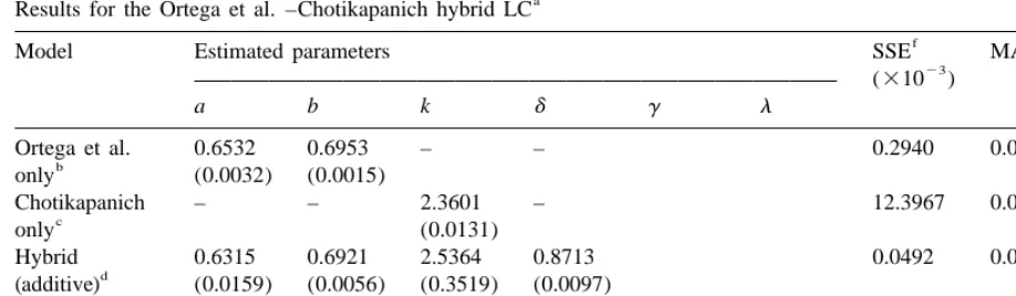
Table 1
a Results for the Ortega et al. –Chotikapanich hybrid LC
f g h
Model Estimated parameters SSE MAVE G
23 (310 )
a b k d g l
Ortega et al. 0.6532 0.6953 – – 0.2940 0.0066 0.370
b
only (0.0032) (0.0015)
Chotikapanich – – 2.3601 – 12.3967 0.0280 0.361
c
only (0.0131)
Hybrid 0.6315 0.6921 2.5364 0.8713 0.0492 0.0044 0.368
d
(additive) (0.0159) (0.0056) (0.3519) (0.0097)
Hybrid 3.0539 3.0309 1.0624 0.4756 0.4411 7.7980 0.0510 0.369
e
Based on the model y5[(exp(kp)21) /(exp(k)21)]. The corresponding expression for the Gini index is [(k22)exp(k)1
(k12)] / [k(exp(k)21)].
SSE denotes the sum of squares of model estimation errors. g
MAVE denotes the maximum absolute value of model estimation errors. h
G denotes the Gini index.
smaller sums of squares of model estimation errors (SSE) and smaller maximum absolute values of model estimation errors (MAVE), where the errors are defined as the difference between the actual income shares and the estimated income shares. In this case the additive hybrid LC performs distinctly better than the individual component LCs. Second, the multiplicative hybrid LC performs slightly worse than the two constituent LCs on the basis of MAVE and slightly better than one of the two constituent models on the basis of SSE. Combining the two observations, we conclude that the additive model performs better than its multiplicative counterpart. Third, the Gini indices associated with the individual constituent models and those based on the two versions of the hybrid model are remarkably similar. Basmann et al. (1990) also used the same data to estimate five models of the LC and found that the corresponding estimates of the Gini index, obtained using numerical integration techniques, ranged from 0.36 to 0.39. Ogwang and Rao (1996) estimated a LC, defined as an arc of an optimal circle, using the same data and obtained an estimate of the Gini index of 0.39. The estimates of the Gini index for the same data, obtained by Ryu and Slottje (1996, p. 266) using Bernstein polynomial approximations and exponential polynomial approximations of the LC are all between
4
0.36 and 0.37, which are remarkably close to our estimates.
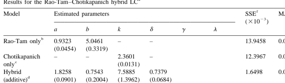
The results for the Rao-Tam–Chotikapanich hybrid LCs, reported in Table 2, indicate that both the additive and multiplicative versions of the Rao-Tam Chotikapanich hybrid LC perform better than either of the constituent LCs in terms of smaller SSEs and MAVEs. Another striking feature of Table 2 is that the additive hybrid LC performs better than its multiplicative counterpart. As in the previous
4
Table 2
Rao-Tam only 0.9323 5.0461 – – 13.9458 0.0301 0.361
(0.0454) (0.3319)
Chotikapanich – – 2.3601 – 12.3967 0.0280 0.361
c
only (0.0131)
Hybrid 1.8258 0.7543 7.5885 0.7379 1.6498 0.0140 0.368
d
(additive) (0.0901) (0.2004) (1.3962) (0.0684)
Hybrid 3.3199 3.3746 4.3765 0.2010 0.3729 12.2525 0.0278 0.362
e
a,21a,ln b), where F denotes the confluent hypergeometric function with parameters (11 1 1a), (21a) and ln b. Note that
` k
F (11a,21a,ln b)5(11a)o [1 /(11a1k)][(ln b) /k!]. However, the series converges so fast that only a few terms
1 1 k5o
of the series expansion are sufficient for accurate estimates of the Gini index to be obtained. c
Based on the model y5[(exp(kp)21) /(exp(k)21)]. The corresponding expression for the Gini index is [(k22)exp(k)1
(k12)] / [k(exp(k)21)].
SSE denotes the sum of squares of model estimation errors. g
MAVE denotes the maximum absolute value of model estimation errors. h
G denotes the Gini index.
case, the Gini indices are very comparable to those obtained by Basmann et al. (1990), Ryu and Slottje (1996), and Ogwang and Rao (1996).
4. Conclusions
In this paper we have proposed hybrid LCs as a way of circumventing an important drawback of traditional models of the LC, namely lack of satisfactory fit over the entire range of a given income distribution. Two categories of hybrid models are identified, namely the additive models and the multiplicative models. Whereas the additive models are obtained by taking convex combinations of the traditional models, the multiplicative models are obtained by taking their weighted products. A comparison of the performances of the hybrid LCs with those of the constituent LCs shows that both the additive and multiplicative models perform generally better than the constituent LCs.
References
Arnold, B.C., 1986. A class of hyperbolic Lorenz curves. Sankhya 48 Series B, 427–436.
Chotikapanich, D., 1993. A comparison of alternative functional forms for the Lorenz curve. Economics Letters 3, 187–192. Gupta, M.R., 1984. Functional forms for fitting the Lorenz curve. Econometrica 52, 1313–1314.
Kakwani, N.C., Podder, N., 1973. On the estimation of Lorenz curves from grouped observations. International Economic Review 14, 278–292.
Kakwani, N.C., Podder, N., 1976. Efficient estimation of the Lorenz curve and the associated inequality measures from grouped data. Econometrica 44, 137–148.
Ogwang, T., Rao, U.L.G., 1996. A new functional form for approximating the Lorenz curve. Economics Letters 52, 21–29. Ortega, P., Martin, G., Fernandez, A., Ladoux, M., Garcia, A., 1991. A new functional form for estimating Lorenz curves.
Review of Income and Wealth 37, 447–452.
Rao, U.L.G., Tam, A.Y., 1987. An empirical study of selection and estimation of alternative models of the Lorenz curve. Journal of Applied Statistics 14, 275–280.
Rasche, R.H., Gaffney, J., Koo, A.Y.C., Obst, N., 1980. Functional forms for estimating the Lorenz curve. Econometrica 48, 1061–1062.
Rossi, J.W., 1985. Notes on a new functional form for the Lorenz curve. Economics Letters 17, 193–197.
Ryu, H.K., Slottje, D.J., 1996. Two flexible functional form approaches for approximating the Lorenz curve. Journal of Econometrics 72, 251–274.
Sarabia, J., 1997. A hierarchy of Lorenz curves based on the generalized Tukey’s lambda distribution. Econometric Reviews 16, 305–320.
Schader, M., Schmid, F., 1994. Fitting parametric Lorenz curves to grouped income distributions–a critical note. Empirical Economics 19, 361–370.
˜