250 (2000) 233–255
www.elsevier.nl / locate / jembe
Estimation of phytoplankton production from space: current
status and future potential of satellite remote sensing
*
Ian Joint , Stephen B. Groom
NERC Centre for Coastal and Marine Sciences, Plymouth Marine Laboratory, Prospect Place, The Hoe, Plymouth PL1 3DH, UK
Abstract
A new generation of ocean colour satellites is now operational, with frequent observation of the global ocean. This paper reviews the potential to estimate marine primary production from satellite images. The procedures involved in retrieving estimates of phytoplankton biomass, as pigment concentrations, are discussed. Algorithms are applied to SeaWiFS ocean colour data to indicate seasonal variations in phytoplankton biomass in the Celtic Sea, on the continental shelf to the south west of the UK. Algorithms to estimate primary production rates from chlorophyll concentration are compared and the advantages and disadvantage discussed. The simplest algorithms utilise correlations between chlorophyll concentration and production rate and one equation is used to estimate daily primary production rates for the western English Channel and Celtic Sea; these estimates compare favourably with published values. Primary production for the central Celtic Sea in the period April to September inclusive is estimated from SeaWiFS data to be
22 22
102 gC m in 1998 and 93 gC m in 1999; published estimates, based on in situ incubations,
22
are ca. 80 gC m . The satellite data demonstrate large variations in primary production between 1998 and 1999, with a significant increase in late summer in 1998 which did not occur in 1999. Errors are quantified for the estimation of primary production from simple algorithms based on satellite-derived chlorophyll concentration. These data show the potential to obtain better estimates of marine primary production than are possible with ship-based methods, with the ability to detect short-lived phytoplankton blooms. In addition, the potential to estimate new production from satellite data is discussed. 2000 Elsevier Science B.V. All rights reserved.
Keywords: Phytoplankton; Primary production; Ocean colour satellites; Celtic Sea; Western English Channel; Chlorophyll concentration
*Corresponding author.
E-mail address: [email protected] (I. Joint).
1. Introduction
There is an urgent need to obtain accurate and precise estimates of global oceanic primary production to solve a number of important environmental problems. For
example, models of the flux of atmospheric CO2 to the oceans depend on accurate
representation of phytoplankton activity in the drawdown of CO ; understanding of the2
limits to marine production and the management of sustainability of marine ecosystems require accurate estimates of phytoplankton production; and the influence of anthro-pogenic inputs of contaminants to the oceans and atmosphere can only be adequately monitored and understood if information is available on a global basis. Classical methods of determining primary production rely on ship-borne observations and experiments. These have been very successful to date in determining the scale of marine primary production but the methodology is intrinsically limited to small space and time scales—and many regions of the ocean have few or no data. The lack of (synoptic) observations means that short-lived events are frequently not sampled. Satellite remote sensing offers the potential for synoptic, global observation of the oceans and could resolve many of the current uncertainties of primary production estimates.
Phytoplankton cells are small with cell dimensions ranging from ,1 mm to a few
tens or perhaps hundredmm. How can they can be measured by a satellite at a distance of hundreds of kilometres—a difference in scale of perhaps 10 orders of magnitude? Of course, individual cells cannot be visualised but, on a typical pixel of 1 km resolution, the signal of phytoplankton pigments is readily detected in satellite images. However, much more important than mere visualisation of distribution patterns have been recent advances which allow accurate quantification of the concentration of those pigments. This has opened up a truly novel field of study, with great potential for biological oceanography.
The advantages of satellites over conventional oceanography are clear: satellites sample over much greater space scales than are possible with ships and at frequencies which are impossible to match by any other sampling procedure. Synoptic sampling at high frequency is now possible over large oceanic regions because a number of ocean colour satellites are now operational.
However, there are also limitations. The most important are that the sea surface is frequently obscured by cloud cover; sunglint masks the surface, as can high levels of aerosol in the atmosphere. Finally, since the satellite signal originates in the surface layer, it is usually not possible to observe sub-surface chlorophyll maxima.
2. Remote sensing of pigment concentration
2.1. Satellite sensors
Satellite instruments measure ocean colour by detecting the upwelling radiance as ‘seen’ through the Earth’s atmosphere in a number of wavebands which correspond to high, medium and low absorption by phytoplankton pigments. A full description of the technology is beyond the scope of this review (see Curran, 1985, for further details) but, briefly, radiance is sampled over the region of the earth’s surface visible in the sensor ‘instantaneous field-of-view’ and contiguous samples are used to construct an image with each sample called a picture-element or pixel.
The first dedicated ocean colour satellite was the Coastal Zone Color Scanner (CZCS) launched by NASA in 1978 and operated intermittently until its failure in 1986 (Mitchell, 1994). As a ‘proof of concept’ mission, CZCS was designed with a number of features specific to ocean colour observation. It viewed the Earth in four narrow wavebands in the visible located in regions of high medium and low phytoplankton absorption; it had high- and variable-gain detectors to allow observation at a variety of solar elevations; and finally it had a mechanism to tilt the observation angle away from the sun to minimise the impact of sunglint. The sensor clearly demonstrated the feasibility of measuring phytoplankton pigment from space to observe spatial variations or temporal variability over weekly monthly, seasonal and yearly timescales (Feldman, 1989). Importantly, the CZCS sensor allowed the first satellite-based estimates of global production (see Longhurst et al., 1995).
Following the end of data acquisition by CZCS, there was 10-year hiatus until the Japanese space agency launched the Ocean Colour and Temperature Sensor (OCTS) in August 1996. OCTS provided ocean colour imagery between November 1996 and June 1997. In August 1997 the sea-viewing wide field-of-view sensor (SeaWiFS) was launched on the Orbview-2 spacecraft. Compared to CZCS the SeaWiFS instrument has been improved in a number of ways. First, it views the Earth in six bands in the visible, including a 412-nm channel to detect coloured dissolved organic matter (CDOM), an additional blue channel at 490 m at medium phytoplankton absorption and two bands in the near infrared to support atmospheric correction (see below). Second, the signal to noise (S /N ) ratio is much higher than CZCS. Finally, the sensor has on-board calibration capabilities. This contrasts with the CZCS which could not be calibrated in-orbit and, since it was designed for a 1-year life, degradation in the system was apparent over the 8 years of operation. On SeaWiFS, short-term variability is checked by daily observations of the sun through a diffuser; longer-term stability is monitored by monthly observations of the moon using the same optical path as the upwelling earth light (Barnes et al., 1999). A limitation to the exploitation of SeaWiFS is that the instrument is operated as a commercial venture, with research use purchased by NASA. Operational and some near real-time applications cannot be supported through NASA and data must be purchased from Orbview.
Table 1
Sensor waveband of three ocean colour sensors which are or have been operational to date; signal to noise characteristics (S /N ) from Esaias et al. (1998)
CZCS S /N SeaWiFS S /N MODIS S /N
waveband (nm) waveband (nm) waveband (nm)
412 CDOM absorption 940 411 CDOM absorption 933
443 260 443 950 442 1325
High, medium 490 High, medium 1156 487 High, medium 1308 520 and low pigment 260 510 and low pigment 1055 530 and low pigment 1385 550 absorption 233 555 absorption 690 547 absorption 1114
665 Chlorophyll 1163
670 143 670 798 677 fluorescence 1265
765 Atmospheric 860 746 Fluorescence baseline 1077 865 correction 670 866 and atmospheric correction 1000
NASA ‘Terra’ satellite. MODIS represents a further leap in capability compared to SeaWiFS (see Table 1) with more wavebands, higher S /N ratio, more complex on-board calibration, and the capability of simultaneous observation of ocean colour and sea-surface temperature. Further instrument launches are planned, including MODIS on ‘Aqua’ in December 2000. This will ensure continuity of ocean colour data, and will provide two observations per day (because Terra and Aqua will pass overhead at 10:30 and 14:30 h local time, respectively). Since MODIS is broadcast continuously (and so can be recorded by anyone with an appropriate receiver) and can be used without any commercial restrictions, arguably it will be the most important ocean colour system over the next decade.
2.2. Atmospheric correction
The principal challenge in measurement of ocean colour is to overcome the influence of the atmosphere which both absorbs (reduces) the water-leaving radiance and scatters light into the sensors field of view, so adding to the water signal. These two effects mean that, at around 440 nm, the atmospheric component may comprise about 95% of the total detected radiance (e.g., Gordon and Wang, 1994). Scattering by atmospheric molecules can be calculated as a function of surface pressure and sun-pixel-sensor geometry and the effect removed. In contrast, scattering by atmospheric aerosols is more problematic due to the spatial and temporal variability and unknown composition. The approach employed for SeaWiFS (and other sensors) is to use measurements in the near-infrared, where the sea-water has high inherent absorption and consequently virtually zero water-leaving radiance, to characterise the aerosols and then use look up tables to extrapolate the aerosol signal to visible wavelengths (Gordon and Wang, 1994). This approach needs to be modified in turbid coastal waters where the near-infrared water signal is not negligible (Moore et al., 1999) while aerosols which absorb are potentially still a problem (Antoine and Morel, 1999). The atmospheric correction may also fail when the solar zenith angle is high, either at high latitudes or in mid-latitude winter.
SeaWiFS the observation angle can be tilted away from the sun, but with MODIS potentially large areas of the swath will be covered by sunglint (Barnes et al., 1998)
2.3. Cloud cover
Cloud cover is the most fundamental limitation to ocean colour observation because it masks the sea-surface. The percentage cloud cover depends upon location and season. A partial solution will be to utilise observations from ocean colour sensors passing over at different times of the day: SeaWiFS passes at local noon while MODIS on the Terra spacecraft will view the same point 90 min earlier, so in the presence of (moving) broken cloud a multi-sensor approach should improve retrieval of information.
2.4. Conversion of water-leaving radiance into pigment
Water and its constituents, such as phytoplankton cells, detrital material, and coloured dissolved organic matter, affect the passage of light by scattering and absorption. By virtue of the optical properties oligotrophic waters have a blue appearance; with increasing phytoplankton concentration, the spectral water-leaving radiance becomes darker and greener (Morel and Prieur, 1977). The wavelength-dependent, water-leaving
l l l l
radiance, L , is proportional to b /ab where bb is the backscatter coefficient (the l
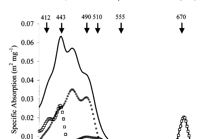
fraction of light scattered by .908 to the incident direction) and a is the absorption coefficient (see Kirk, 1994, for definitions and discussion). The ability to detect phytoplankton from space relies on the spectral variation in phytoplankton pigment absorption (Fig. 1 shows the high absorption in the blue and low in the green region of the spectrum (Aiken et al., 1995)). The spectral structure of chlorophyll-specific absorption (that is absorption normalised to chlorophyll a concentration) varies depend-ing on the composition of the phytoplankton pigments present (Hoepffner and Sathyendranath, 1991) and the magnitude of absorption varies between species due the size of the phytoplankton cells and other factors related to packaging effects (Geider and Osborne, 1992). Empirical and semi-analytic approaches have been used to retrieve phytoplankton pigment concentration from the water signal. The empirical approach
green blue green blue blue
commonly uses ratios of green to blue radiance (i.e., L /L |bb /bb ?a /
green
a )—the radiance in the blue decreases with increasing pigment concentration—while
the green may slightly increase due to scattering. Furthermore, by taking a ratio, the magnitude differences in absorption and scattering (as opposed to spectral variation) are partly cancelled. The semi-analytic approach utilises a more complete description of the optical properties of phytoplankton and associated detrital material (e.g., Carder et al., 1999; Ciotti et al., 1999) to retrieve chlorophyll concentration.
2.5. Case II waters
Fig. 1. Specific absorption due to all pigments (—), chlorophyll a (h), photosynthetic carotenoids (s) and
photoprotective carotenoids (^); data modified from Aiken et al. (1995). The wavelengths of the SeaWiFS wavebands are indicated.
waters—but in many cases, phytoplankton standing stock is low. Suspended particulate matter (SPM), either re-suspended from the bottom or of fluvial origin, and CDOM originating from river outflow have a large influence on existing chlorophyll retrieval algorithms. In these regions, estimation of chlorophyll concentration using existing empirical algorithms is problematic: the influence of SPM and CDOM will change the parameters in the empirical relationships while the RMS error for retrievals may also be higher (see Mitchelson et al., 1986). Furthermore, the techniques of retrieving the water signal from the satellite detected radiance may fail (Moore et al., 1999). There is a need for novel modelling approaches to determine the inherent optical properties of scattering and absorption from remotely sensed observations. Until that time, the estimation of pigment concentration, and hence of phytoplankton production, in Case II waters will be problematic.
2.6. Sub-surface chlorophyll maxima
Estimates are limited to the near surface and ocean colour sensors will only detect pigments within one optical depth (that is, the depth at which surface irradiance is attenuated to 1 / e537% of its surface intensity). In order to convey information about phytoplankton at this depth the light must then pass back through the water column and
2
phyto-plankton assemblages within a subsurface chlorophyll maximum and hence biomass will 23
be underestimated. For example, for a surface concentration of 0.5 mg m , the optical depth for PAR is |11 m (Berthon and Morel, 1992): for a chlorophyll profile with 0.5
23 23 23
mg m 0#Z#10, increasing to 1.0 mg m at 15 m and 2.0 mg m at 20 m, the
23
satellite will sense chlorophyll |0.56 mg m compared to a mean value of 0.85 mg
23
m for the upper 20 m.
3. Estimation of primary production from pigment concentration
Satellite remote sensing gives an estimate of photosynthetic pigment concentrations near to the sea surface. An important question for biological oceanographers is to determine if this information can be used to give accurate and precise estimates of primary production. It is perhaps counter-intuitive that primary production (with
3 3
dimensions of ML T) should be derived only from an estimate of standing stock (ML ). It could be argued that the rate of carbon fixation by any particular phytoplankton biomass might be dependent on factors other than the amount of pigment present; nutrient limitation, depth distribution of biomass in the water column and temperature might all be expected to influence the rate of primary production. However, it appears that these processes have little influence on production estimates and a great deal of progress has been made in estimating primary production from pigment concentration alone (Behrenfeld and Falkowski, 1997b).
Models which have been applied to satellite remote sensing have basically been of two types—empirical and semi-analytical (Behrenfeld et al., 1998). Those which estimate production from standing stock are essentially empirical. They may be influenced by local conditions, and it is possible that they can only be applied to those oceanic provinces for which the algorithms were originally derived; that is, these relationships may prove to be geographically specific. In an attempt to obtain globally applicable models, more complex algorithms have been developed which utilise knowledge of physiological response and light absorption properties. Both empirical and semi-analytical models have advantages and disadvantages.
3.1. Empirical models
(1957) was an important demonstration that reasonable estimates of primary production (in this case determined by oxygen evolution) could be made from a knowledge of chlorophyll concentration, extinction coefficient and light.
Research in the intervening four decades has demonstrated that primary production can indeed be estimated successfully from chlorophyll concentration. The simplest
14
methods have involved regressions of C uptake rates against chlorophyll concentration. For example, Eppley et al. (1985) in an analysis of 10 datasets from a wide range of ocean provinces, found a clear relationship between depth-integrated primary production
22 21 23
(mg C m day ) and near-surface chlorophyll concentration (mg m ). The
relationship was not linear and they suggested that there might be regional differences in the production-chlorophyll relationship and that this could also vary with time of year. However, seasonality may be a relatively minor component of the variance in chlorophyll / primary production relationships. In an analysis of data for the Southern California Bight, Eppley et al. (1985) found that the seasonal effect accounted for |9%
of total variance. For another dataset based on samples taken from the end of Scripps pier, Eppley et al. (1985) again showed the importance of chlorophyll concentration which explained 33% of the variance in production estimates; day length and sea surface temperature anomaly explained 23% of the remaining variance. So the simplest possible approach of utilising the relationship between chlorophyll concentration and primary production would appear to have considerable potential for remote sensing applications. More complex empirical relationships have been suggested. One of the most robust
was by Falkowski (1981) who suggested that the slope (C) of chlorophyll-specific,
21 21
depth-integrated production against light had a constant value of 0.43 g C g Chl Ein 22
m (where 1 Ein is 1 mol quanta). Jordan and Joint (1984), in a seasonal study of the
English Channel foundCto have a value of 0.48, and suggested thatCmay be constant in different oceanic provinces. Platt (1986) reviewed eight different data sets and
21 21 22
commented on the narrow range of estimates ofC(0.31–0.66 g C g Chl Ein m )
for these different studies. However, the relationship does not appear to be universal and other measurements, such as those by Yoder et al. (1985) in the South Atlantic Bight, and Balch et al. (1989) in the Southern California Bight, found poor correlations.
Perhaps the most promising approach to date is the model suggested by Behrenfeld and Falkowski (1997a). This is a light-dependent, depth-independent model which requires a small number of parameters. Depth-integrated primary production, PP , iseu
B
estimated from the following: Popt, the maximum rate of chlorophyll-specific carbon fixation in the water column; E , sea surface daily photosynthetically available radiationo
(PAR); Z , the depth of water from the surface to where light is 1% of that at theeu B
surface; Copt, the chlorophyll concentration at the depth at which Poptoccurs; and D, the number of hours of daylight on that day. This simple model explained 86% of the variance between measured and modelled production estimates for a very large data set of nearly 1700 estimates of primary production from a number of marine provinces. The
B
limitation in this model is that when Poptwas estimated from a parameter available from remote sensing (sea-surface temperature) the variance explained dropped to 58%.
derived—although further research is required to determine the extent of the variability and whether it is predictable. Nevertheless, the empirical approach has great potential to be easily applied to the latest generation of ocean colour satellites. In a later section of this paper, we will use a simple empirical relationship to explore seasonal variations in primary production for the Celtic Sea shelf and English Channel.
3.2. Semi-analytical models
The second approach to the problem of estimating primary production has been to derive algorithms which might have wide application and could be usefully applied to the global ocean. These models involve increased complexity by incorporating a higher level understanding of biological processes and of light distribution in the water column. There are many such models (Behrenfeld and Falkowski, 1997b), but two of the best known are by Platt et al. (1990, 1991) and Morel (1991). It is not appropriate in this paper to review these models in detail but the essence of the approach is to use
B
chlorophyll-specific photosynthesis versus irradiance (P /E ) parameters to estimate production from modelled light and chlorophyll vertical distributions.
The advantage of these algorithms is that they are based on an understanding of the way in which photosynthesis and phytoplankton adapt and respond to the light field in the sea and to the factors which determine light availability at any depth in the euphotic zone. Disadvantages are that many determinations of the photosynthesis / irradiance
B
relationship are required to provide the basic data for the models and P /E parameters can only be derived experimentally and, in contrast to pigment concentration, are not retrievable directly from satellite imagery.
3.3. Consideration of errors
It is appropriate to consider the error that can be expected, the predictability, and the performance, when primary production algorithms is estimated with remotely sensed data. Balch et al. (1989) investigated the performance of empirical algorithms, noting that the Eppley et al. (1985) algorithm performed best: regression of predicted against
2
observed daily integrated production gave r 50.38, increasing to 0.42 when
satellite-14
derived pigment was used. Behrenfeld and Falkowski (1997a) used a compilation of C
data to show that a product of surface chlorophyll and euphotic depth explained 38% of variance in PPeu or 29% for log transformed data. (The euphotic depth can be retrieved from the attenuation coefficient, K: the attenuation coefficient at 490 nm is a standard SeaWiFS product.) The Behrenfeld and Falkowski (1997a) vertically generalised
B
production model with Popt calculated from surface temperature explained 58% of the
observed variance in integrated production (or 53% for log transformed data). Using the simple algorithm given in Behrenfeld et al. (1998):
log10PP50.559 log10C12.793. (1)
2
(log10PPmodel50.739 log10PPin situ10.689, R 50.75).
The relatively high explained variance may imply that there is little uncertainty in satellite derived production estimates. However, a more appropriate statistic is the predictability or spread in data around the regression line that can be expected for a given value of C. Considering an equation of the form (1), there is 95% confidence that a future observation of y5log10PP at x05log10C for some specified C lies in the0 0
where a and b are the fitted regression parameters, syux is the residual standard
deviation, t0.025,n22is the percentage point of Student’s t distribution for n22 degrees of freedom, and hx ; ii 51 . . . nj are the log10C values used in fitting the regression
equation. This is known as the prediction interval.
The spread of the predicted value will depend on the statistics of the regression line in Eq. (1) and the uncertainty in the retrieval of satellite quantities. The error in satellite-retrieved chlorophyll from the CZCS in the western English Channel was approximately 0.26 log10C (Holligan et al., 1983). Preliminary results from SeaWiFS in
situ validation (Kahru and Mitchell, 1999) give a similar RMS error as a result of uncertainty in the in situ empirical algorithms (for example, O’Reilly et al., 1998) and the error in the atmospheric correction. In order to estimate prediction intervals, data for the Celtic Sea have been fitted with a regression similar to Eq. (1) giving:
log10PP50.567 log10C12.83 (2)
The 95% prediction interval is60.26 log10PP at the mean chlorophyll concentration of 23
log10C5 20.25 or C50.56 mg m ; this will increase as values diverge from the
mean. If the error in satellite derived chlorophyll is60.3 log10C, then calculation of the
prediction interval at mean chlorophyll gives an overall prediction interval of 60.43
22 21
log10PP. That is, at the mean value of production of|0.6 gC m day corresponding
23
to mean chlorophyll (0.56 mgm ), there is 95% probability that the predicted value will 22 21
lie between 0.33 and 1.1 gC m day if the retrieved chlorophyll concentration has no
22 21
error, or between 0.22 and 1.6 gC m day if the error in chlorophyll is60.3 log10C.
Conversely, if the relationship between primary production and chlorophyll were exact
2
(i.e., r 51) then the 95% predicted interval would give primary production between 0.4
22 21
and 0.88 gC m day , the range being due to uncertainty in chlorophyll retrieval.
Clearly the uncertainty in the primary production / chlorophyll algorithm is the primary source of error in satellite retrieval. Furthermore, it is expected that the SeaWiFS retrievals of chlorophyll should be improved with developments in retrieval algorithms and atmospheric correction procedures.
paper. However, given that similar errors will occur in the measurement of other
B
biological parameters such as the photosynthesis—irradiance parameters (a and P ) andm
the phytoplankton spectral absorption, it is reasonable to suppose that the additional complexity will increase the error in model predictive capability.
Errors may arise through the use of simple models in regions or biogeochemical provinces not represented in the data sets used to construct the relations. For example, the regression statistics for data from the Celtic Sea have been used as opposed to the (unknown) statistics in the Behrenfeld et al. (1998) algorithm. Use of the latter would cause even greater spread in the prediction interval. Similarly, significant errors would arise in the use of inappropriate values in the more detailed algorithms using province-based approaches (e.g., Longhurst et al., 1995).
4. The Celtic Sea and English Channel as a case study: estimation of annual phytoplankton production
In this section, we highlight a region of shelf sea to the south west of the UK which includes the English Channel and Celtic Sea. The English Channel has been the subject of oceanographic study for almost 120 years and many advances in marine science were made here. For example, the earliest measurements of nutrient concentration in the sea were done in the coastal waters off Plymouth by Matthews (1917), who developed methodology to measure phosphate concentration. Yet in spite of the many years of study, there are few seasonal estimates of primary production (Jordan and Joint, 1984) and poor understanding of interannual variability. Algorithms have been applied to data from the SeaWiFS ocean colour sensor in the English Channel and compared with estimates of primary production previously made in the summer months of 1981. Similar comparisons are made for a second site, in the Celtic Sea, for which seasonal estimates of primary production are also available (Joint and Pomroy, 1983; Joint et al., 1986).
4.1. Seasonal changes in ocean colour
Fig. 2. Pseudo-natural image based on a composite of bands from the SeaWiFS colour sensor. (a) 20 March 1998, (b) 18 May 1998, (c) 8 August 1998 and (d) 20 September 1998.
By mid-summer, phytoplankton pigment concentrations are reduced and most of the central Celtic Sea appears to be blue (Fig. 2c). At this time of year, Joint and Pomroy
(1983) found that most of the production was by small phytoplankton cells ,5 mm;
indeed almost half of the production was by picophytoplankton ,1 mm. The contrast
between well mixed and stratified waters is very obvious. The east of the English Channel and Bristol Channel are well mixed and maintain high concentrations of suspended particles which result in enhanced scattering. In this image, there was cloud, notably west of the Bristol Channel and northwest of Brittany, which is represented as black. The late summer image (Fig. 2d) shows a remarkable degree of structure which is difficult to interpret. There is high absorption along the front between mixed and stratified waters which runs north from Ushant to the south English coast. At this time of year, stratification is beginning to break down and this may result in enhanced flux of nutrients from the deep, tidally mixed layer into the euphotic zone, with an enhancement of primary production. We have no field data with which to test these ideas but the image is a useful illustration of how satellite remote sensing can reveal features in the surface ocean which require further investigation and field measurements.
4.2. Chlorophyll concentration in the Celtic Sea and western English Channel
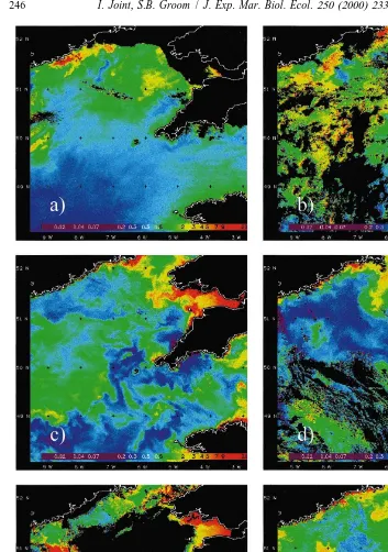
The images in Fig. 2 demonstrate the complex nature of seasonal changes in water colour in the Celtic Sea and show the occurrence of specific events such as coc-colithophore blooms. Fig. 3 is a series of false colour SeaWiFS images showing chlorophyll concentration at six times of the year from late March to late September. SeaWiFS chlorophyll retrievals are calculated from a ratio of the 490- and 555-nm bands with the NASA OC2 version 2 algorithm (O’Reilly et al., 1998). The 490-nm band is used, rather than 443 nm, where chlorophyll absorption is higher, since the absorption by CDOM is lower at the higher wavelength and there is usually a strong correlation between the chlorophyll a and carotenoids, the latter being the main absorbing pigments at 490 nm, (Aiken et al., 1995). As already mentioned, there are considerable difficulties in estimating chlorophyll concentration in waters with high suspended particulate concentrations. Comparison of Fig. 3c with Fig. 2b illustrates the problem: chlorophyll retrieval algorithms estimate high pigment concentrations in the Bristol Channel where the suspended sediments resulted in high reflectance (Fig. 2b). Similar problems exist in the east of the English Channel visible in these images. However, most of the region has Case I waters, with low concentrations of suspended particles and CDOM and precise estimates of chlorophyll concentration are possible.
Fig. 3a shows estimated chlorophyll concentration for the region on 20 March. The area of dark water off the Irish coast in Fig. 2a is now indicated as a region of high (ca.
23
5 mg m ) chlorophyll concentration but most of the region has chlorophyll
con-23
centration of much less than 1?5 mg m . By 26 April (Fig. 3b) phytoplankton biomass has increased considerably and most of the region has chlorophyll concentrations of 2
23 23
mg m ; there are many patches where concentrations are .5 mg m . Fig. 3c shows
Fig. 3. False colour SeaWiFS images of estimated chlorophyll concentration in the surface waters of the Celtic Sea: (a) 20 March 1998, (b) 26 April 1998, (c) 18 May 1998, (d) 15 June 1998, (e) 8 August 1998 and (f) 20
23
always the case and coccolithophore blooms in other provinces do not always have high chlorophyll concentration associated with high reflectance. Chlorophyll concentrations in the surface waters begin to decline from mid June (Fig. 3d) and by 8 August, most of
23
the region has concentrations considerably less than 0.5 mg m (Fig. 3e). This image
shows the clear effect of islands in enhancing phytoplankton biomass (Simpson et al., 1982), with higher chlorophyll concentrations round the Isles of Scilly, off the tip of Cornwall. The image of 20 September (Fig. 3f) indicates that chlorophyll concentrations have again increased in a late summer bloom of phytoplankton, with concentrations up
23
to 3 mg m .
4.3. Estimation of annual production: comparison with previous estimates for the
Celtic Sea and western English Channel
Fig. 3 has shown the utility of SeaWiFS to provide excellent spatial and temporal coverage of pigment concentrations in the Celtic Sea. We now consider the potential for estimating primary production from these estimates of chlorophyll concentration. Two stations in the Celtic Sea region are used for which seasonal estimates of primary production are available. Station E1 (508029N: 48229W) in the western English Channel was the focus of a study of primary production by Jordan and Joint (1984) and seasonal production estimates are published for station CS2 (508309N: 078009W) in the central Celtic Sea (Joint and Pomroy, 1983; Joint et al., 1986).
The algorithm of Behrenfeld et al. (1998) discussed above has been tested for the English Channel by applying it to the chlorophyll data of Jordan and Joint (1984) to give estimates of primary production which can be compared with the rates measured by Jordan and Joint (1984). However, such comparison is not straightforward because different timescales apply. Jordan and Joint (1984) did short-term (,5 h incubations)
14 22 21
using the C method and results are given as mgC fixed m h . Daily estimates of
primary production computed with Eq. (1) and surface chlorophyll concentration give estimates of daily production which are less than half the daily rate (PP ) calculated byJJ
multiplying the hourly estimates of Jordan and Joint by the photoperiod (e.g., Balch et al., 1989). Primary production is estimated from Eq. (1)
2
(PPeqn1)50.41 PPJJ1138.82 (r 50.79, n59).
The hourly rates of Jordan and Joint (1984) are normalised by the average irradiance experienced over the incubations, which were done around midday; this is much higher irradiance than would be experienced throughout the entire photoperiod when light limitation would be expected. Scaling the day length by the ratio of average irradiance over the incubation period by the average over the whole photoperiod gives
2
PPeqn150.61 PPJJ91137.42 (r 50.80, n59).
Daily estimates of primary production obtained by extrapolating the hourly estimates of Jordan and Joint to 24 h (PP ,) still gives a higher estimates than Eq. (1) because theyJJ
a 24-h incubation. Williams and Lefevre (1996) point out the importance of excretion of labelled organic matter and of respiration in 24-h incubations. If these could be taken into account, the difference between daily primary production estimates from Eq. (1) and from hourly production estimates could be further reduced. This exercise highlights that there are frequently problems when using compilations of data from different investigators to validate production algorithms.
Eq. (1) has been applied to chlorophyll data retrieved from SeaWiFS to give estimates of primary production at two time scales. Fig. 4 shows monthly estimates of primary production for the western English Channel and central Celtic Sea. These charts have been produced by compositing over each month daily images of primary production calculated from daily chlorophyll concentration. This approach has the advantage that the effects of cloud cover can be minimised because any partial image can contribute information to the monthly composite and so it is more likely that estimates can be obtained for the whole region of interest. The disadvantage is that short-lived events can bias the monthly average. The second approach (Fig. 5) shows daily estimates for regions surrounding stations in the English Channel in 1998 and 1999. Estimates are restricted to the period from March to September since the presence SPM affects chlorophyll retrievals October–March, while the low sun-angle causes problems with the atmospheric correction over a similar period. Each point is a mean with error bars showing standard deviation of the six pixels surrounding ‘Station 1’ (Jordan and Joint, 1984). The proximity to the coast means that the variability in chlorophyll is considerable. In both 1998 and 1999, production increased in the spring; in 1998 there was a late summer increase in production which did not occur in 1999. Primary production of the English Channel for the period April to September inclusive is
22 22
estimated to be 122 gC m in 1998 and 124 gC m in 1999.
Fig. 6 shows similar estimates for the region of the Celtic Sea including station CS2. Again there were significant difference between years, with a late summer increase in production in 1998 which did not occur in 1999. The estimated primary production for
22 22
April to September is 102 gC m in 1998 and 93 gC m in 1999. Joint et al. (1986)
estimated monthly and annual primary production for station CS2 in the Celtic Sea. For the period April to September inclusive, they estimated primary production to be 80 gC
22
m , although they had no measurements for September which was estimated by
Fig. 4. Primary production estimated from composite chlorophyll distributions for (a) April, (b) May, (c) June,
22 (d) July, (e) August and (f) September 1998. The colours corresponding to primary production (mgC m
21
Fig. 5. Daily primary production in the English Channel estimated from SeaWiFS images in a) 1998 and b) 1999.
5. The additional potential of satellite remote sensing
5.1. New production and limits to productivity
Fig. 6. Daily primary production in the Celtic Sea estimated from SeaWiFS images in a) 1998 and b) 1999.
ammonium and it increases asymptotically with increasing nitrate concentration. Satellite imagery has been applied to the problem of estimating new production. Sathyendranath et al. (1991) showed that surface nitrate concentration was correlated with temperature in the surface waters of Georges Bank. Recently, Dugdale et al. (1997) have used sea surface temperatures as a proxy to model surface nitrate distributions. So it is well established that, for certain times and locations, it is possible to use sea surface temperatures, derived from the AVHRR sensor, to map nitrate distributions over large areas of the surface ocean.
con-centration, it has been possible to get estimates for the f ratio for Georges Bank (Sathyendranath et al., 1991) and for the Goban Spur region of the Celtic Sea shelf break (Joint et al., 2000).
5.2. Estimation of other biogeochemical parameters
A number of novel algorithms have been suggested to utilise remote sensing to investigate additional biogeochemical variables. For example, the flux of CO from the2
atmosphere to the ocean is poorly quantified on a global basis. The partial pressure of
CO2 in the surface ocean has been measured from ships but Aiken et al. (1992)
suggested that p(CO ) could be assessed by aircraft remote sensing. Changes in p(CO )2 2
depend on temperature and the activity of marine microbes, with reduction being found in regions of high phytoplankton biomass and production. Therefore, chlorophyll concentration and temperature, two parameters which are readily measured by remote sensing, should be correlated with p(CO ). Aiken et al. (1992) found a relationship2
which could be applied to aircraft remote sensing and which explained 71% of the
variance in p(CO ). Although this study used aircraft remote sensing, Aiken et al.2
highlighted the potential for satellite imagery to improve understanding of the role of the oceans in understanding of the global carbon cycle.
6. Future developments
We are at the very early stages of exploiting the potential of satellite remote sensing to determine marine productivity. Ocean colour satellites have only been operational for a couple of years and already chlorophyll and production have been estimated in provinces for which little or no field observations existed. With the launch of the first MODIS instrument on ‘Terra’ and the forthcoming launch of a second sensor on ‘Aqua’, data on ocean colour should continue to be available for the immediate and medium-term future. The additional wavebands of the MODIS sensors will provide the opportunity to improve the algorithms for chlorophyll concentration retrieval. In particular, it should be possible to improve on the current empirical algorithms for estimating pigment concentration and to move to semi-analytical approaches.
There is scope for novel research with MODIS to find out if it is possible to use the waveband at 677 nm (and the ‘baseline’ bands at 665 and 746 nm) to determine chlorophyll fluorescence from space (Neville and Gower, 1977). If this ambitious objective is attained, then alternative methods for estimating primary production could be possible. Other important research will investigate the potential for detecting different phytoplankton taxa. With the increased number of wavebands available, information on different accessory pigments could be sufficient to indicate the dominant organisms in a phytoplankton bloom.
All these advances will depend on additional experiments and observations at sea. It should be possible to improve the precision of satellite estimates of phytoplankton biomass and production. However, precision is not the same as accuracy and these
14
production. In spite of nearly 50 years of use, there are still large uncertainties associated
14
with C primary production estimates (Williams and Lefevre, 1996). As highlighted
above, it can be very difficult to compare one data set with another; short-term incubations of a few hours do not necessarily relate well to estimates based on longer incubations of 12 or 24 h. Variations in methodology make comparisons difficult between different researchers. So, although we will soon be able to reduce the variance of satellite-based estimates, it may be some time before a consensus is reached on how accurately these estimates reflect the actual global marine primary production.
Acknowledgements
This research forms part of the Core Strategic Research Project on the Dynamics of Marine Ecosystems (DYME) of the Centre for Coastal and Marine Sciences, Plymouth Marine Laboratory. The research was partially funded by the NERC Thematic Programme on Marine Productivity (GST / 02 / 2765). We are very grateful to Dr. K.R. Clarke for advice on statistical treatment of error propagation. [RW]
References
Aiken, J., Moore, G.F., Holligan, P.M., 1992. Remote sensing of oceanic biology in relation to global climate change. J. Phycol. 28, 579–590.
Aiken, J., Moore, G.F., Trees, C.C., Hooker, S.B., Clark, D.K., 1995. In: Hooker, S.B., Firestone, E.R. (Eds.), The SeaWiFS CZCS-type pigment algorithm. NASA Technical Memorandum 104566, Vol. 29, NASA Goddard Space Flight Center, Greenbelt, MD, USA.
Antoine, D., Morel, A., 1999. A multiple scattering algorithm for atmospheric correction of remotely sensed ocean colour (MERIS instrument): principle and implementation for atmospheres carrying various aerosols including absorbing ones. Int. J. Remote Sens. 20, 1875–1916.
Balch, W.M., Abbott, M.R., Eppley, R.W., 1989. Remote sensing of primary production. I. A comparison of empirical and semi-analytical algorithms. Deep-Sea Res. 36, 281–295.
Barnes, W.L., Pagano, T.L., Salomonson, V.V., 1998. Pre-launch characteristics of the Moderate Resolution Imaging Spectrometer (MODIS) on EOS-AM1. IEEE Trans. Geosci. Remote Sens. 36, 1088–1100B. Barnes, R.A., Eplee, R.E., Patt, F.S., McClain, C.R., 1999. Changes in the radiometric sensitivity of SeaWiFS
determined from lunar and solar-based measurements. Appl. Optics 38, 4649–4664.
Behrenfeld, M.J., Falkowski, P.G., 1997a. Photosynthetic rates derived from satellite-based chlorophyll concentration. Limnol. Oceanogr. 42, 1–20.
Behrenfeld, M.J., Falkowski, P.G., 1997b. A consumer’s guide to phytoplankton primary production models. Limnol. Oceanogr. 42, 1479–1491.
Behrenfeld, M.J., Falkowski, P.G., Esaias, W.E., Balch, W., Campbell, J.W., Iverson, R.L., Kiefer, D.A., Morel, A., Yoder, J.A., 1998. Towards a consensus productivity algorithm for SeaWiFS. In: Hooker, S.B., Firestone, E.R. (Eds.), SeaWiFS Technical Report Series, Vol. 42, Satellite primary productivity data and algorithm development: a science plan for Mission to Planet Earth. Goddard Space Flight Center, Greenbelt, MD, USA, pp. 18–25.
Berthon, J.F., Morel, A., 1992. Validation of a spectral light-photosynthesis model and use of the model in conjunction with remotely sensed pigment observations. Limnol. Oceanogr. 37, 781–796.
Ciotti, A.M., Cullen, J.J., Lewis, M.R., 1999. A semi-analytical model of the influence of phytoplankton community structure on the relationship between light attenuation and ocean color. J. Geophys. Res. 104, 1559–1578.
Curran, P.J., 1985. In: Principles of Remote Sensing. Longman, Harlow.
Dugdale, R.C., Goering, J.J., 1967. Uptake of new and regenerated forms of nitrogen in primary productivity. Limnol. Oceanogr. 12, 196–206.
Dugdale, R.C., Davis, C.O., Wilkerson, F.P., 1997. Assessment of new production at the upwelling center at Point Conception, California, using nitrate estimated from remotely sensed sea surface temperature. J. Geophys. Res. 102, 8573–8585.
Elskens, M., Goeyens, L., Dehairs, F., Rees, A., Joint, I., Baeyens, W., 1999. Improved estimation of f-ratio in natural phytoplankton assemblages. Deep-Sea Res. 46, 1793–1808.
Eppley, R.W., Peterson, B.J., 1979. Particulate organic matter flux and new production in the deep ocean. Nature 282, 677–680.
Eppley, R.W., Stewart, E., Abbot, M.R., Heyman, V., 1985. Estimating primary production from satellite chlorophyll: introduction to regional differences and statistics for the Southern California Bight. J. Plankt. Res. 7, 57–70.
Esaias, W.E., Abbott, M.R., Barton, I., Brown, O.B., Campbell, J.W., Carder, K.L., Clark, D.K., Evans, R.H., Hoge, F.E., Gordon, H.R., Balch, W.M., Letelier, R., Minnett, P.J., 1998. An overview of MODIS capabilities for ocean science observations. IEEE Trans. Geosci. Remote Sens. 36, 1250–1265. Falkowski, P.G., 1981. Light-shade adaptation and assimilation numbers. J. Plankt. Res. 3, 203–217. Feldman, G.C., 1989. Ocean color, availability of the global data set. EOS Trans. AGU 70, 634–641. Garcia Soto, C., Fernandez, E., Pingree, R.D., Harbour, D.S., 1995. Evolution and structure of a shelf
coccolithophore bloom in the western English Channel. J. Plankt. Res. 17, 2011–2036.
Geider, R.J., Osborne, B.A., 1992. In: Algal Photosynthesis. Chapman and Hall, New York, p. 256 pp. Gordon, H.R., Wang, M.H., 1994. Retrieval of water-leaving radiance and aerosol optical thickness over the
oceans with SeaWiFS: a preliminary algorithm. Appl. Optics 33, 443–452.
Hoepffner, N., Sathyendranath, S., 1991. Effect of pigment composition on absorption properties of phytoplankton. Mar. Ecol. Prog. Ser. 73, 11–23.
Holligan, P.M., Viollier, M., Dupouy, C., Aiken, J., 1983. Satellite studies on the distributions of chlorophyll and dinoflagellate blooms in the western English Channel. Cont. Shelf Res. 2, 81–96.
Joint, I.R., Pomroy, A.J., 1983. Production of picoplankton and small nanoplankton in the Celtic Sea. Mar. Biol. 77, 19–27.
Joint, I.R., Owens, N.J.P., Pomroy, A.J., 1986. Seasonal production of photosynthetic picoplankton and nanoplankton in the Celtic Sea. Ecol. Prog. Ser. 28, 251–258.
Joint, I., Wollast, R., Chou, L., Batten, S., Elskens, M., Edwards, E., Hirst, A., Burkill, P., Groom, S., Gibb, S., Miller, A., Hydes, D., Dehairs, F., Antia, A., Barlow, R., Rees, A., Pomroy, A., Brockmann, U., Cummings, D., Lampitt, R., Loijens, M., Mantoura, F., Miller, P., Raabe, T., Alvarez-Salgado, X., Stelfox, C., Woolfenden, J., 2000. Pelagic production at the Celtic Sea Shelf Break—the OMEX I project. Deep Sea Res. II (in press).
Jordan, M.B., Joint, I.R., 1984. Studies on phytoplankton distribution and primary production in the western English Channel in 1980 and 1981. Cont. Shelf Res. 3, 25–34.
Kahru, M., Mitchell, B.G., 1999. Empirical chlorophyll algorithm and preliminary SeaWiFS validation for the California Current. Int. J. Remote. Sens. 20, 3423–3429.
Kirk, J.T.O., 1994. Estimation of the absorption and the scattering coefficients of natural waters by use of underwater irradiance measurements. Appl. Optics 33, 3276–3278.
Longhurst, A., Sathyendranath, S., Platt, T., Caverhill, C., 1995. An estimate of global primary production in the ocean from satellite radiometer data. J. Plankt. Res. 17, 1245–1271.
Matthews, D.J., 1917. On the amount of phosphoric acid in the sea water of Plymouth Sound. I and II. J. Mar. Biol. Assoc. UK 11, 122–30, 251–257.
Mitchell, B.G., 1994. Coastal zone color scanner retrospective. J. Geophys. Res. 99, 7291–7292.
Mitchelson, E.G., Jacob, N.J., Simpson, J.H., 1986. Ocean colour algorithms from the Case 2 waters of the Irish Sea in comparison to algorithms from Case 1 waters. Cont. Shelf Res. 5, 403–415.
Morel, A., 1991. Light and marine photosynthesis: a spectral model with geochemical and climatological implications. Prog. Oceanogr. 26, 263–306.
Morel, A., Prieur, L., 1977. Analysis of variations in ocean color. Limnol. Oceanogr 22, 709–722. Neville, R.A., Gower, J.F.R., 1977. Passive remote sensing of phytoplankton via chlorophyllafluorescence. J.
Geophys. Res. 82, 3487–3493.
O’Reilly, J.E., Maritorena, S., Mitchell, B.G., Siegel, D.A., Carder, K.L., Garver, S.A., Kahru, M., McClain, C., 1998. Ocean color chlorophyll algorithms for SeaWiFS. J. Geophys. Res. 103 (C11), 24937–24953. Platt, T., 1986. Primary production of the ocean water column as a function of surface light intensity.
Deep-Sea Res. 33, 149–163.
Platt, T., Sathyendranath, S., Ravindran, P., 1990. Primary production by phytoplankton: analytic solutions for daily rates per unit area of water surface. Proc. R. Soc. London B. 241, 101–111.
Platt, T., Caverhill, C., Sathyendranath, S., 1991. Basin-scale estimates of oceanic primary production by remote sensing: the North Atlantic. J. Geophys. Res. 96, 15147–15159.
Ryther, J.H., Yentsch, C.S., 1957. The estimation of phytoplankton production in the ocean from chlorophyll and light data. Limnol. Oceanogr. 2, 281–285.
Sathyendranath, S., Platt, T., Horne, E.P.W., Harrison, W.G., Ulloa, O., Outerbridge, R., Hoepffner, N., 1991. Estimation of new production in the ocean by compound remote sensing. Nature 353, 129–133. Simpson, J.H., Tett, P.B., Argote-Espinoza, M.L., Edwards, A., Jones, K.J., Savidge, G., 1982. Mixing and
phytoplankton growth around an island in a stratified sea. Cont. Shelf Res. 1, 15–31. 14
Williams, P.J., Lefevre, D., 1996. Algal C and total carbon metabolisms. 1. Models to account for the physiological processes of respiration and recycling. J. Plankt Res. 18, 1941–1959.