WHY THE HORIZON IS IMPORTANT FOR AIRBORNE SENSE AND AVOID
APPLICATIONS
Cyrus Minwalla∗, Kristopher Ellis
Flight Research Laboratory, National Research Council Canada, Ottawa, ON, Canada - (cyrus.minwalla, kristopher.ellis)@nrc.ca
KEY WORDS:SAA, ABSAA, UAS, horizon model, horizon proximity, region-of-interest, feature detector
ABSTRACT:
The utility of the horizon for airborne sense-and-avoid (ABSAA) applications is explored in this work. The horizon is a feature boundary across which an airborne scene can be separated into surface and sky and serves as a salient, heading-independent feature that may be mapped into an electro-optical sensor. The virtual horizon as established in this paper represents the horizon that would be seen assuming a featureless earth model and infinite visibility and is distinct from the apparent horizon in an imaging sensor or the pilot’s eye. For level flight, non-maneuvering collision course trajectories, it is expected that targets of interest will appear in close proximity to this virtual horizon. This paper presents a model for establishing the virtual horizon and its projection into a camera reference plane as part of the sensing element in an ABSAA system. Evaluation of the model was performed on a benchmark dataset of airborne collision geometries flown at the National Research Council (NRC) using the Cerberus camera array. The model was compared against ground truth flight test data collected using high accuracy inertial navigation systems aboard aircraft on several ’near-miss’ intercepts. The paper establishes the concept of ’virtual horizon proximity’ (VHP), the minimum distance from a detected target and the virtual horizon, and investigates the utility of using this metric as a means of rejecting false positive detections, and increasing range at first detection through the use of a region of interest (ROI) mask centred on the virtual horizon. The use of this horizon-centred ROI was shown to increase the range at first detection by an average factor of two, and was shown to reduce false positives for six popular feature detector algorithms applied across the suite of flight test imagery.
1. INTRODUCTION
The global market for small unmanned aircraft systems (UAS) is expected to grow significantly over the next decade [Mendel-son, 2014]. Building inspections, pipeline monitoring and aerial photography/videography production are among the success sto-ries for commercial applications utilizing UAS, as they can be performed within visual line of sight of the pilot. It is more diffi-cult to gain approval of flight operations beyond the visual line of sight (BVLOS), owing to the regulatory requirement to see and avoid conflicting air traffic. This requirement either restricts BV-LOS operations to segregated, or unpopular airspace (e.g. low level over the ocean, or arctic), or necessitates the use of a sense and avoid (SAA) system with an equivalent level of safety to the manned aircraft see and avoid principle. Regulatory bodies have yet to establish a consensus on the required performance stan-dard for a sense and avoid system, however several groups are currently working on solutions to this issue, with the most re-cent developments revolving around a specified target level of safety that is comparable to that of the current mid-air collision rate for manned aircraft. Despite the lack of performance stan-dards, the SAA problem has been the subject of a vast amount of academic, commercial and regulatory activity and still remains an open problem for operations in civil airspace.
2. BACKGROUND
An airborne SAA (ABSAA) system based on electro-optical (EO) or infrared (IR) cameras must transform a sequence of images into an accurate and reliable estimate of collision-course targets. The standard approach to the problem is a detection and tracking pipeline consisting of the extraction of ’good’ features, followed by tracking of those features across the image sequence, and fi-nally, applying target discrimination criteria to remove false pos-itives.
∗Correspondence author
2.1 Electro-Optical SAA Techniques
Aircraft
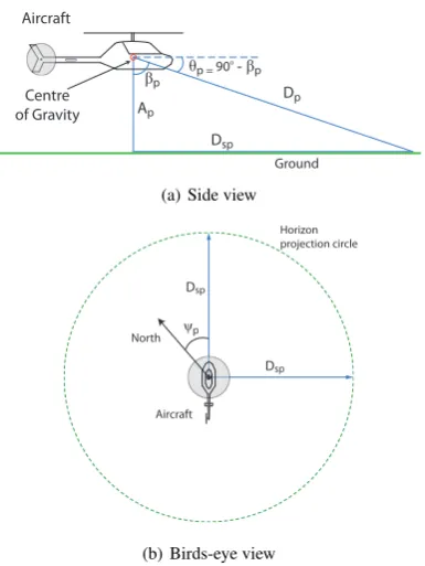
Figure 1: Side and birds-eye views of the theoretical horizon on the Earth’s surface.
in hardware on an unmanned helicopter. They compared the per-formance of Harris and Shi-Tomasi feature detectors against syn-thetic targets. Here, we present the results of those corner de-tectors, among others, against real targets acquired from airborne near-collision flights.
3. MODEL
This section describes the theoretical horizon model and its pro-jection, defined as the “virtual horizon” into an electro-optical sense calibrated with respect to the platform INS. The accuracy of the projection is a function of the fidelity of the model, and the precision of the calibration and the INS.
3.1 Inertial Reference Horizon
The theoretical horizon defines an omnipresent feature that may be used for image stabilization, attitude registration and target lo-calization. Note that it is distinct from a ‘horizon’ that may be visible in the image. In forward-facing imagery acquired at gen-eral aviation altitudes under clear sky assumptions, the horizon is routinely observed to possess a smooth gradient rather than a sharp discontinuity near the ground-sky boundary. This ‘gray’ re-gion is a direct consequence of atmospheric effects and illustrates the complexity of extracting the horizon contour using purely im-age processing techniques. Without an obvious boundary, imim-age processing techniques may be influenced by scene structure and cloud cover to detect a false horizon contour, and are not con-sidered as reliable as a theoretical horizon computed from the platform INS measurements. Previous efforts based on machine learning techniques extracted the contour defined by the ground-horizon boundary [Minwalla et al., 2011]. Such a contour can reveal geological and man-made topological features that a theo-retical horizon will not capture, and may prove useful when fly-ing at low altitudes in a city or near rocky terrain. The approach described in this paper does not tackle those issues and is more suited for general aviation altitudes at 1000 feet or above over roughly level terrain, where the horizon is distant and indistinct.
3.2 Target Behaviour Under ABSAA
A typical intruder for ABSAA is an aircraft encountered in non-segregated airspace that will spend the majority of flight time under non-maneuvering and non-accelerating conditions. Such aircraft are likely to appear at or near the horizon. Targets that appear above the virtual horizon are sky-lit and are expected to have greater contrast than those that appear at or below the vir-tual horizon. Targets that appear below the virvir-tual horizon are difficult to distinguish from ground clutter, and prove to be the most challenging targets. However, for all oncoming cases where one aircraft appears below the horizon, the other aircraft will ob-serve the host as a high-contrast sky-lit target above the horizon. This is not the case in descending overtake scenarios, where the aircraft being overtaken cannot see the overtaking aircraft due to a limited cockpit field of view. This suggests that descending over-take scenarios are the most difficult to detect. Looking at these non-co-altitude cases will form part of future work.
3.3 Derivation
We start the description of the model with the assumption that the Earth is an ellipsoid devoid of topological features. At a given platform altitude, the distance to the horizon (Dp) is defined by
a line from the aircraft centre of gravity to a point tangent to the ellipsoid. This line forms a right-angled triangle between the air-craft centre, the tangent point and the centre of the Earth. Fig. 1(a) depicts the direct linear distance to the horizon asDp, while
Dspdepicts the corresponding ground-track distance andApis
the platform local above ground level (AGL). The INS reference frame origin is placed at the aircraft’s centre of gravity.
Apand the local earth radius,Rp, are the only two quantities
required to ascertainDp,Dspand the declination angle (θp) (Eq.
Note that atmospheric scattering will limit the visibility to well withinDp, referred to asDp′. By contrast, atmospheric
refrac-tion will extend the distance to beyondDp, referred to asD′′p.
Therefore, D′
p < Dp < D′′p. Since atmospheric scattering is
the limiting factor, the apparent horizon in real, forward-facing imagery is typically closer, atD′
p, and by extension, positioned
lower in pixel coordinates. Note thatDspcan be treated similarly.
If perceived from a birds-eye configuration, the horizon projects a circle of radiusDspon the earth’s ellipsoidal surface, centred
at the aircraft position (Fig. 1(b)). Assume that the position,
Xp = [Xp, Yp, Zp,1]and the attitude,[θp, φp, ψp], of the host
platform are known in a local Cartesian coordinate system. One such Cartesian system is the local Universal Transverse Mercator (UTM). Since the radius of the circle,Dsp, is strictly a function
of the platform altitude, points on the horizon circle (Xh) are
relative to the platform position and can be represented in the host aircraft inertial reference frame (Eq. 2).
Xh(α) = Here, ψpdenotes the heading of the aircraft. The azimuth, α,
model may be used to project body axis coordinates into image space. For convenience, we use the pinhole camera model in our work. Although not explicitly explored, this model may be aug-mented for distortion correction if necessary. Eq. 3 denotes the projection matrix, whereKis the intrinsic matrix,[Rc| −Rctc]
the fixed calibration between the camera and the aircraft INS, and
[Rv| −Rvtv]the INS to world transformation.
x=PX, whereP=K·[Rc| −Rctc]·[Rv| −Rvtv] (3)
The world horizon points may be projected into the camera plane as per Eq. 4:
xh= [u,v,w]T=PXh,where
w >0
1≤u≤nrows
1≤v≤ncols
(4)
The horizon circle may be sampled at equidistant intervals ofα and projected into image coordinates. The points of interest, de-noted byxh(Eq. 4), are those that possess valid image
coordi-nates and are in front of the camera, the latter property defined by a positive magnitude inw. Note thatnrowsandncolsrefers to the row and column pixel counts of the focal plane array respectively. At least two suitable points are needed, therefore the sampling in-terval forα, denoted asταmust be at leastF OV ≥2ταwhere
F OV is the camera’s field of view.
Note that this solution is applicable regardless of the camera ori-entation and is readily expanded to multiple cameras, indepen-dently or serially calibrated to the aircraft INS reference frame.
3.4 Virtual Horizon Proximity (VHP) -∆Htgt
Given the projection of a virtual horizon line in image coordi-nates, the virtual horizon proximity (VHP) is defined as the dis-tance between a potential target and the virtual horizon line. The VHP concept exploits a characteristic unique to level-flight, col-lision course targets, namely their quasi-constant separation from the horizon for the duration of the course. This cue is strictly a function of the altitude difference between the host and intruder platforms and is invariant to the host and target attitudes. Given the horizon line,∆Htgtmay be computed by the distance
equa-tion (Eq. 5), wherext is the target point,xh
1 and x
h
2 are two points from the projected horizon line.
∆Htgt=
(xi−xh
1)×(x
i−xh
2)
|xh
2−xh1 |
(5)
To validate the VHP hypothesis, the measured intruder proximity (Htgt) must be compared to a ground-truth estimate from known
host and intruder positions. This estimate can be generated as fol-lows: Let us assume a plane parallel to the camera plane located at the intruder that defines the background. As the intruder is much closer than the theoretical horizon, the distant horizon line must be projected onto this background plane coincident with the intruder. Retaining the ellipsoid assumption, letHp=Rp+Ap
andHi = Ri+Ai, whereRpandApare as before,Aiis the
intruder altitude andRi is the local ellipsoidal radius at the
in-truder. Then the ground-truth proximity in radians,∆ ˆHtgt, can
be derived via similar triangles and the cosine law (Eq. 6),
β= acos
H2
p+D2i −Hi2
2DiHp
θ= acos
H2
p+D2p−Hi2
2DpHi
∆ ˆHtgt= (β−θ)/F OVpix
(6)
(a) Raw image
(b) After ROI weighting
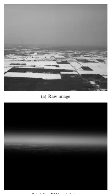
Figure 2: An image from a head-on collision couse with the March 2012 dataset with and without a ROI applied. The Bell 206 acted as the intruder. The image dimensions are 2448 columns by 2050 rows for reference. The ROI mask was generated by a Gaus-sian PDF centred at the horizon with a half-width of 150 pixels.
Here,Dpis the distance from the platform to the horizon (from
Eq. 1) andDi the distance between the host and the intruder.
ThisHˆtgtmodel is utilized for ground-truth estimates in Section
5.. Note that Dp >> Di for general aviation altitudes. For
instance, at an altitude of 300 m (Ap= 1000ft), distance to the
horizon is≈60km. Furthermore, the projective relationship is reasonable at long ranges, whereDi>> fandfis the lens focal
length. At close ranges, the assumptions begin to break down and parallax effects limit the efficacy of this technique.
3.5 Horizon-weighted Region-of-Interest Mask
The primary purpose of a region-of-interest (ROI) mask is to re-duce clutter and false positives by isolating the pixels where the target of interest is likely to appear. A typical ROI is a rectangu-lar crop with a step function weighting, such that pixels outside the region are eliminated. Although the rectangular ROI is fast to compute, it has the unfortunate side-effect of culling all tar-gets that may occur outside the expected region of interest. We propose the use of a horizon-weighted ROI mask as a target like-lihood estimator. This weighted ROI can be implemented as a spatial probability density function (PDF) centred at the virtual horizon and applied perpendicularly to the direction of the hori-zon line.
(a) Host - Bell 205
(b) Intruder - Bell 206
(c) Intruder - Harvard Mark IV
Figure 3: Host and intruder aircraft used for airborne near-collision flight tests.
positives from the scene clutter have a reduced impact. Fig. 2(a) illustrates a raw capture during a head-on collision run. In Fig. 2(b), a Gaussian PDF with a half-width of 150 pixels and centred at the horizon line, is applied as a weighting mask. The choice of function, bias and half-width are user-configurable parameters and can be tailored to the host platform’s performance envelope, although care must be taken as too narrow an ROI or too steep a gradient may result in target drop-outs.
4. EXPERIMENTS
4.1 Airborne Flight Tests
Flight tests were flown with a Bell 205 helicopter acting as a sur-rogate UAS (Fig. 3(a)) [Ellis and Gubbels, 2005]. A Bell 206 ro-torcraft (Fig. 3(b)) and a Harvard Mark IV trainer fixed-wing air-craft (Fig. 3(c)) acted as the intruders. Flights were flown in con-trolled airspace near the Flight Research Laboratory at Ottawa In-ternational Airport (CYOW). Common test conditions consisted of visual meteorological conditions (VMC) at high visibility in excess of 15 statute miles (24 km). Tests were conducted in the morning and afternoon to encounter different solar zenith an-gles. Each sortie consisted of 6-10 collision geometries, where each collision geometry was flown from∼15km separation to within 100 meters. Data was collected on head-on, azimuthal off-set, chase, descending head-on and descending overtake trajecto-ries. The aircraft were instrumented with an automatic dependent surveillance-broadcast (ADS-B) transceiver and an INS [Leach et al., 2003]. An “Intercept Display”, parsing the on-board ADS-B
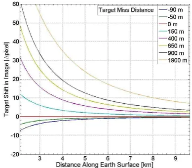
Figure 4: Modeled temporal VHP for collision course targets at different relative altitudes to the host platform. Nominal altitude was set to 1000 ft. “Target Miss Distance” indicates the altitude differential in metres between the host and each intruder.
data, provided range and navigation guidance to the flight crew for beyond visual line of sight operation [Keillor et al., 2011].
4.2 Instrument Configuration
A multi-camera array, dubbed Cerberus, was rigidly mounted to the port-side external mount of the Bell 205. Each imager con-sisted of a 5 megapixel monochrome sensor operating at 15 fps. Monochrome sensors were chosen to enhance focal plane reso-lution at the expense of colour fidelity. A fixed-focal-length lens was installed per camera. The images were streamed over Ether-net to a local rack-mount PC, where each frame was synchronized via GPS time-stamp to the precision INS on board the Bell 205 and recorded for offline analysis. The total instrument field-of-view nominally spanned 90-degrees from the forward look direc-tion, with subsequent flights conducted with a variety of sensor and lens configurations.
4.3 Selection of Benchmark Data
Although a considerable number of trajectories were flown, only a selected subset of the data is presented for analysis and com-parison. These benchmark datasets were chosen for their clar-ity of the imagery, similar sensor configuration and favourable scene conditions (high visibility, minimal cloud cover and oc-clusions). A total of four collision trajectories were chosen for analysis: three head-on and one azimuthal offset. Head-on colli-sions represent the scenario limiting critical problem-space, due to a maximal closure rate and a minimal observable intruder foot-print. All frames of interest were acquired with the same forward-facing camera to correlate the sensor noise characteristics across datasets. Specific parameters for the flight tests are outlined in Table 4. while relevant Cerberus parameters are presented in Ta-ble 4..
Date and Time Intruder Ground Visibility Altitude Geometry Host Heading
[km] [ft±2σ] [deg±2σ]
July 8 2009
Harvard Mk IV Farmland 24 2000±500 Head-On 273±4
13:00 - 14:00 EST 10◦Offset 105±8
Mar 7 2012
Bell 206 Snow 24 2000±500 Head-On 1 236±2
9:00 - 10:00 EST Head-On 2 246±2
Table 1: Benchmark Datasets from July 2009 and March 2012
Parameter Value Units
July 2009 March 2012
Cameras 3 2
-Azimuth configuration (0◦,45◦,90◦) (0◦,45◦) deg Total FOV 113◦×34◦ 75◦×(18◦,50◦) deg
Focal length (f) 12 0◦=23,45◦=8 mm
Focal ratio (F#) 4.0 (0◦,45◦)=2.8
-Angular resolution 0.3 0◦=0.15,45◦=0.43 mrad/pixel Focal plane dimensions 2448×2050 (×3) 2448×2050(×2) pixels
Table 2: Cerberus Array Parameters
into a target visible at greater ranges at the expense of field of view.
5. RESULTS AND DISCUSSION
5.1 Temporal VHP -∆Htgt(t)
The target VHP measured over a sequence of images is expected to indicate co-altitude collision-course behaviour. Fig. 4 presents the behaviour of a MATLAB model simulating level -flight col-lision -course intruders approaching a host UAS at various alti-tude differentials. The abscissa denotes range while the ordinate depicts the VHP as a function of range. Here, range is used in-terchangeably with time by assuming a constant closing velocity. It can be observed that the absolute VHP is directly correlated to the altitude differential, with larger VHP indicating larger correc-tions. Furthermore, as the intruder approaches the host, the VHP grows non-linearly for all cases except the co-altitude one. This indicates that a small absolute VHP value and minimal temporal variation are both indicators of collision-course behaviour.
To experimentally verify this phenomenon, we compare the mea-sured VHP (Htgt) to the ground-truth VHP (Hˆtgt) derived in Eq.
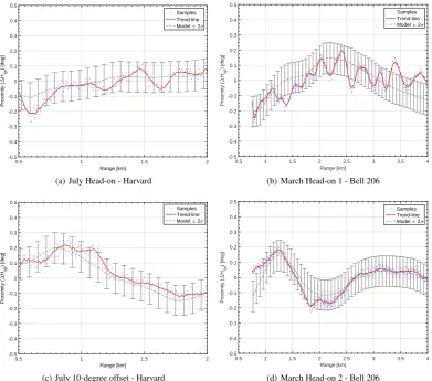
6. Recall that the ground-truth VHP is the height differential ex-tracted from the INS data recorded on-board host and intruder aircraft. Fig. 5 contains the VHP plots acquired from the July and March datasets respectively. In each curve, the abscissa is the range and the ordinate is the proximity to the projected hori-zon measured in degrees. Points represent the per-frame VHP (Eq. 5) converted into degrees via the known camera scale factor. A trend-line is depicted to enhance readability. The dotted grey line illustrates the modeled proximity derived in Section 3.4, with error bars indicating the±2σ = 0.1deg error in the on-board INS attitude measurements of the host and intruders [Leach et al., 2003].
It is observed that the measured VHP tracks the model consis-tently for the duration of the flight geometry in all four plots. Plots for both intruder types are on track, demonstrating the ro-bustness of the cue against variations in the intruder radiance pro-file. In addition, the heading offset has no impact on the mea-surement (Figs. 5(a) and 5(c)). However, two different head-on collision trajectories flown within a few minutes of each other can exhibit different temporal VHP profiles (Figs. 5(b) and 5(d)). Periodic oscillations are present in the measured proximity val-ues for July Head-on and March Head-on 1 (Figs. 5(a) and 5(b))
that are not explained by the models, or visible in July Offset or March Head-on 2 geometries (Figs. 5(c) and 5(d)). It is spec-ulated that these perturbations are tied to INS drift correction, suggesting that optical methods could be utilized to augment atti-tude measurements. Once again, the observed effect is minor and the peak-peak variation remains well within the2σbounds of the INS error.
Note that the deviation between measured and modeled proximity curves will increase at close ranges due to parallax. A breakdown of the assumption is visible in Fig. 5(d) but not obvious in the other plots. Table 5.1 summarizes the plot results. Note that the absolute deviation is miniscule, with the maximum peak-to-peak variation limited to0.51degrees (observed in March Head-On 1). The maximum deviation from the model is0.35degrees ob-served in March Head-On 2 (Fig. 5(b)). For all intents and pur-poses,∆Htgt(R)is roughly constant. In summary,∆Htgt(R)
is a quasi-constant cue for collision-course targets, consistent be-tween trajectories and is robust against changes in the intruder type, radiance profile and background clutter.
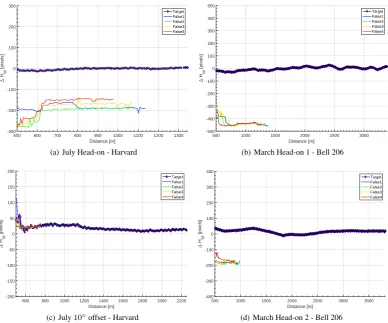
5.2 Comparison to False Positives
To observe the proximity effect, we compare the temporal VHP of the known, true target against other false positives detected in the scene. Target detection and tracking was implemented via al-gorithms developed locally at NRC. These alal-gorithms rely on vi-sual cues unique to collision course targets augmented by Kalman filtering for a robust, real-time estimation.
Fig. 5.3 illustrates the proximity plots of the ground-truth target and four other highest-likelihood false positives. The abscissa denotes the range while the ordinate denotes the virtual horizon proximity (VHP) measured in pixel coordinates. The diamond markers show the true target while false positives are indicated by coloured lines. It is observed that all detected false positives are below the horizon, corresponding to false targets embedded in ground clutter. The true target has the minimum distance to the virtual horizon line (smallest|∆Htgt|) and maintains
Range [km]
(a) July Head-on - Harvard
Range [km]
(c) July 10-degree offset - Harvard
Range [km]
Figure 5: Temporal VHP profiles from the July 2009 and March 2012 datasets. Individual data points (in blue) represent the per-frame VHP (Eq. 5) converted into degrees via the known camera scale factor. A trend-line (in red) is shown to enhance readability. The dotted grey line with error bars illustrates the modeled proximity (Eq. 6). The height of the error bars is derived from the±2σ= 0.1
deg error in the on-board INS attitude measurements.
Aircraft Trajectory Peak-Peak [deg] Max Deviation [deg]
Harvard Head-on 0.51 0.15
10◦Offset 0.32 0.14
Bell 206 Head-on 1 0.52 0.21
Head-on 2 0.46 0.35
Table 3: Peak-Peak variation between predicted and measured virtual horizon proximity (VFP)
intruders, one co-altitude and one not, is required to demonstrate the utility of temporal VPH in discriminating between a collision-course and a non-collision-collision-course intruder. However, such data is not available yet and is relegated to future work. Note that the overlap of multiple targets at close range in Fig. 6(c) is an ar-tifact of the track estimation algorithm currently under develop-ment and has little bearing on the analysis.
5.3 Detection Performance of Weighted ROI Mask
Since a region-of-interest limits the scene to areas of interest, it stands to reason that horizon-weighted ROI masks can lead to fewer false positives and consequently a greater range at earliest detection (Rdet). Six popular feature detectors were compared to
determine the impact of ROI weighting onRdet. Seven feature
detectors were identified in prior work [Tulpan et al., 2014], of which the following six were chosen for comparison: FAST [Ros-ten et al., 2010], Shi-Tomasi [Shi and Tomasi, 1994], Harris-Plessey [Harris and Stephens, 1988], MSER [Matas et al., 2004], SIFT [Lowe, 2004] and SURF [Bay et al., 2006]. Detector im-plementations were sourced from the OpenCV library version
2.4.9 (64-bit) and interfaced into MATLAB via themexopencv
API [Yamaguchi, 2015]. The actual range values are expected to be slightly different from prior work due to the differences in feature detector settings and the OpenCV version. Nonetheless, the overall trend is expected to be consistent.
Table 5.3 contains the results of this comparison. All four bench-mark datasets were tested against the six algorithms. The number of features detected per frame was restricted to 50, and the ROI mask was chosen to be a Gaussian PDF at a half-width of 150 pix-els centred at the virtual horizon line. Each element of the table denotes the range at earliest detection,Rdet, in units of
kilome-tres, as observed for that dataset-algorithm-weighted/unweighted combination. The performance improvement is generally posi-tive across all chosen algorithms with a weighted ROI. The effect is significant in some cases (July 10◦-offset and March Head-on 1) and almost negligible in others (March Head-Head-on 2). The degree of variability bears further investigation. The FAST al-gorithm performed the best and posted the greatestRdet values
Distance [m]
500 600 700 800 900 1000 1100 1200 1300
"
(a) July Head-on - Harvard
Distance [m]
500 1000 1500 2000 2500 3000
"
600 800 1000 1200 1400 1600 1800 2000 2200
"
500 1000 1500 2000 2500 3000 3500
"
Figure 6: Comparison of true target proximity to false positives tracked across the image sequence. The abscissa denotes the range while the ordinate denotes the virtual horizon proximity (VHP) measured in pixel coordinates. Top five targets are presented. The true target, indicated by diamond markers, is observed to have the smallest| ∆Htgt |and maintains quasi-static proximity to the virtual
horizon in all four datasets. The false positives have a greater|∆Htgt|, but are also quasi-static with thscene.
Detector Harvard - Head-on Harvard -10
◦Offset Bell 206 - Head-on 1 Bell 206 - Head-on 2
No ROI 150-pixel No ROI 150-pixel No ROI 150-pixel No ROI 150-pixel
FAST 3.197 4.937 1.229 4.044 3.291 7.249 1.569 1.619
Shi-Tomasi 1.404 4.778 1.127 3.259 2.803 5.390 1.569 1.569
Harris 0.965 4.723 1.086 3.225 2.417 5.180 1.569 1.569
MSER - 0.964 0.817 0.893 - 1.572 -
-SIFT 0.984 2.287 0.906 1.940 1.546 2.378 1.569 1.569
SURF 0.943 0.943 0.865 1.264 0.164 2.270 -
-Table 4: The range at earliest detection,Rdet, with and without a weighted ROI Mask. Each row indicates anRdetvalue kilometres
for that feature detector. Columns indicate the datasets, evaluated with and without the ROI mask. A Gaussian PDF with a half-width of 150-pixels was used to generate the ROI.
cases where the algorithm could not pick up the true target at all. The highest incidence of failure was observed with MSER, sug-gesting that it is a remarkably poor candidate for airborne target detection. The SURF algorithm also failed for the March Head-on 2 dataset. It is noted that use of the ROI mask shifted MSER performance from failure to marginal success in two out of four cases.
6. CONCLUSION AND FUTURE WORK
Presented here is the rationale that the horizon is an important feature for ABSAA applications. A model for the virtual horizon line was presented as a projection of the INS horizon into im-age coordinates. Proximity to the virtual horizon could then be calculated and denoted as the virtual horizon proximity (VHP). The model was tested against simulation results and augmented by local Earth radius corrections for small-angle sensitivity. The
predictions of the model were experimentally verified against a benchmark dataset of collision-course trajectories flown at the National Research Council’s Flight Research Laboratory. An ROI mask, centred at the horizon, was explored as a mechanism for improving the earliest detection range,Rdet. This hypothesis was
experimentally verified by measuring the performance of six pop-ular feature detectors with and without the ROI mask. It was ob-served that the use of the ROI universally improvedRdetacross
all feature detectors and all datasets, sometimes by a factor of two, and in two cases, recovered targets where the feature detec-tor failed in the unweighted case.
ACKNOWLEDGEMENTS
and Fazel Famili for their work on the original analysis.
REFERENCES
Bay, H., Tuytelaars, T. and Gool, L. V., 2006. SURF: Speeded up robust features. In: Proc. European Conference on Computer Vision (ECCV), pp. 404–417.
Carnie, R., Walker, R. and Corke, P., 2006. Image process-ing algorithms for uav “sense and avoid”. In: Proc. IEEE In-ternational Conference on Robotics and Automation, Orlando, Florida, pp. 2848–2853.
Dey, D., Geyer, C., Singh, S. and Digioia, M., 2009. Passive, long-range detection of aircraft: Towards a field deployable Sense and Avoid System. In: Proc. Conference on Field and Service Robotics, pp. 1–10.
Dey, D., Geyer, C., Singh, S. and Digioia, M., 2011. A Cascaded Method to Detect Aircraft in Video Imagery. International Jour-nal of Robotics Research 30(12), pp. 1527–1540.
Ellis, K. and Gubbels, A. W., 2005. The National Research Coun-cil of Canada’s Surrogate UAV FaCoun-cility. In: Proc. UVS Canada Conference.
Fasano, G., Accardo, D., Tirri, A. E., Moccia, A. and Lellis, E. D., 2014. Morphological Filtering and Target Tracking for Vision-based UAS Sense and Avoid. In: Proc. International Con-ference on Unmanned Aircraft Systems, pp. 430–440.
Fasano, G., Moccia, A., Accardo, D. and Rispoli, A., 2008. Development and Test of an Integrated Sensor System for Au-tonomous Collision Avoidance. In: Proc. International Congress of the Aeronautical Sciences, pp. 1–10.
Forlenza, L., Carton, P., Accardo, D., Fasano, G. and Moccia, A., 2012. Real Time Corner Detection for Miniaturized Electro-Optical Sensors Onboard Small Unmanned Aerial Systems. Sen-sors (Basel, Switzerland) 12(1), pp. 863–77.
Harris, C. and Stephens, M., 1988. A Combined Corner and Edge Detector. Proc. Alvey Vision Conference pp. 23.1–23.6.
Keillor, J., Ellis, K., Craig, G., Rozovski, D. and Erdos, R., 2011. Studying Collision Avoidance by Nearly Colliding: A Flight Test Evaluation. In: Proc. Human Factors and Ergonomics Annual Meeting, pp. 41–45.
Lai, J., Ford, J. J., Mejias, L. and O’Shea, P., 2013. Characteri-zation of Sky-region Morphological-temporal Airborne Collision Detection. Journal of Field Robotics 30(2), pp. 171–193.
Leach, B. W., Dillon, J. and Rahbari, R., 2003. Operational experience with optimal integration of low-cost inertial sensors and GPS for flight test requirements. Canadian Aeronautics and Space Journal 49(2), pp. 41–54.
Lowe, D. G., 2004. Distinctive Image Features from Scale-Invariant Keypoints. International Journal of Computer Vision (IJCV) 60(2), pp. 91–110.
Matas, J., Chum, O., Urban, M. and Pajdla, T., 2004. Robust wide-baseline stereo from maximally stable extremal regions. Image and Vision Computing 22(10), pp. 761–767. British Ma-chine Vision Computing 2002.
Mendelson, J., 2014. Innovations in Unmanned Vehicles - Land, Air, Sea (Technical Insights). Technical Report D56B-01, Frost and Sullivan.
Minwalla, C., Watters, K., Thomas, P., Hornsey, R., Ellis, K. and Jennings, S., 2011. Horizon extraction in an optical collision avoidance sensor. In: Proc. Canadian Conference on Electrical and Computer Engineering.
Rosten, E., Porter, R. and Drummond, T., 2010. Faster and Better: A Machine Learning Approach to Corner Detection. IEEE Trans. Pattern Anal. Mach. Intell. (PAMI) 32(1), pp. 105–119.
Salazar, L. R., Sabatini, R., Ramasamy, S. and Gardi, A., 2013. A Novel System for Non-Cooperative UAV Sense-And-Avoid. In: Proc. European Navigation Conference, pp. 1–11.
Shi, J. and Tomasi, C., 1994. Good features to track. In: Proc. IEEE Conference on Computer Vision and Pattern Recognition, pp. 593–600.
Tulpan, D., Belacel, N., Famili, F. and Ellis, K., 2014. Exper-imental evaluation of four feature detection methods for close range and distant airborne targets for Unmanned Aircraft Systems applications. In: Proc. International Conference on Unmanned Aircraft Systems (ICUAS), IEEE, pp. 1267–1273.
Yamaguchi, K., 2015. Mex OpenCV Library.https://github.