Agricultural Economics 23 (2000) 1–15
Short and long-run returns to agricultural R&D in South Africa,
or will the real rate of return please stand up?
David Schimmelpfennig
a,∗, Colin Thirtle
b, Johan van Zyl
c, Carlos Arnade
d, Yougesh Khatri
eaEconomic Research Service, US Department of Agriculture, Washington, DC 20036-5831, USA bUniversity of Reading, and University of Pretoria, Reading, UK
cUniversity of Pretoria, Pretoria, South Africa
dEconomic Research Service, US Department of Agriculture, Moscow, Russia eInternational Monetary Fund, Washington, DC, USA
Received 1 December 1997; received in revised form 29 October 1999; accepted 14 December 1999
Abstract
This paper briefly presents the results of a total factor productivity (TFP) study of South African commercial agriculture, for 1947–1997, and illustrates some potential pitfalls in rate of return to research (ROR) calculations. The lag between R&D and TFP is analyzed and found to be only 9 years, with a pronounced negative skew, reflecting the adaptive focus of the South African system. The two-stage approach gives a massive ROR of 170%. The predetermined lag parameters are then used in modeling the knowledge stock, to refine the estimates of the ROR from short- and long-run dual profit functions. In the short run, with the capital inputs treated as fixed, the ROR is a more reasonable 44%. In the long run, with adjustment of the capital stocks, it rises to 113%, which would reflect the fact that new technology is embodied in the capital items. However, the long-run model raises a new problem since capital stock adjustment takes 11 years, 2 years longer than the lag between R&D and TFP. If this is assumed to be the correct lag, the ROR falls to 58%, a best estimate. The paper draws attention to the possible sensitivity of rate of return calculations to assumed lag structure, particularly when the lag between changes in R&D and TFP is skewed. © 2000 Elsevier Science B.V. All rights reserved.
Keywords: South Africa; TFP; Returns to agricultural R&D; Profit function
1. Introduction
Equivalent measures of technological change exist which are based on the dual relationships between the production, cost and profit functions. These measures are also equivalent to economic accounting measures, based on index number theory. Similarly, there are two econometric approaches to explain changes in agricultural productivity, which form the basis for
∗Corresponding author. Tel.:+1-202-694-5507.
E-mail address: [email protected] (D. Schimmelpfennig)
calculating the returns to research (ROR).1 Evenson et al. (1987) call these the integrated approach (where the productivity-enhancing, or conditioning factors are included directly in a primal or dual representa-tion of producrepresenta-tion) and the two-stage decomposirepresenta-tion, in which changes in total factor productivity (TFP) are first calculated, and then explained, by the condi-tioning factors that are thought to account for growth.
1 There is a huge literature on the returns to agricultural research. See, for example, Echeverria (1990) or Thirtle and Bottomley (1992).
In either case, changes in output, costs, profits, or TFP are usually explained by conditioning vari-ables such as the stock of knowledge (accumulated research capital, generated by past research expen-ditures), extension services and farmer education, as well as changes in the weather. The basic argument is that R&D generates technology, extension diffuses it, and better-educated farmers are better at screening new technology. Consequently, they adopt technolo-gies more quickly and also adapt technology, thereby adding an element of on-farm technology generation. For South Africa, spillovers through international technology transfers are also important, so interna-tional patents are included. Finally, the influence of the weather is considerable, so a weather index should reduce the unexplained errors.
Both integrated and two-stage approaches have ad-vantages and disadad-vantages. The dual integrated ap-proach has the advantage of minimizing restrictive separability assumptions, as well as avoiding the need for the assumptions of full static equilibrium, Hicks neutral technical change, and constant returns to scale, all of which are implicit in the two-stage approach. On the other hand, the two-stage method concentrates on the technology-related variables, so they can be modeled more satisfactorily. Thus, both routes are fol-lowed in this paper, which summarizes and develops the past work in this area with respect to South Africa. The primary focus of the paper is in illustrating some potential pitfalls in ROR calculations. Little at-tention is generally paid to correct lag length and shape parameters in the ROR literature, which are here found to be entirely different from the symmetric structures used previously and this is shown to change the ROR substantially. This result indicates the sensitivity of these ROR calculations to assumed lag structure, espe-cially when the effects of agricultural R&D are skewed and have short lags as in South Africa’s applied and adaptive research system.
Subsequent sections of the paper review the litera-ture on the calculation of South African commercial TFP, and the necessary theory underlying short- and long-run generalized quadratic (GQ) residual profit functions. The rest of the required data, including in-ternational technology spillover variables, and their sources are then discussed, followed by the estimation, results, and calculation of ROR. In conclusion, we in-dicate some possible refinements to agricultural ROR
calculations, without suggesting that the best methods are at hand.
2. TFP growth: 1947–1997
Thirtle et al. (1993) analyze TFP growth in South African agriculture for the period 1947–1992, using a Tornqvist–Theil index. The series has been updated to 1997 by Nick Vink at the University of Stellenbosch, in South Africa. Fig. 1 shows that the output index has grown by over 250% for the period, an annual rate of 2.8%. The index of inputs has more than doubled, growing at 1.5% a year, but considering the entire time period at once hides the fact that inputs grew at over 2.5% per annum until 1979 and since then have been falling at 0.5% per annum. This fall in inputs explains the recent growth in the TFP index. Over the full period, TFP grows rather slowly, at 1.2% per year, but there was no growth until 1965, then 2.13% per annum until 1983, a severe drought year, and a slower growth of 1.5% per annum since 1984.
To explain the causes of the aggregate TFP changes, it is necessary to look at the components of the index. Output can be decomposed into crops, hor-ticulture and fruit, and animal products. Fruit and horticulture have grown more rapidly than crop out-put, while livestock outputs have grown the least. The growth rates were 3.9, 2.7 and 2.3%, respectively, and as a result, the share of horticulture and fruit has increased at the expense of the other enterprises. The indices behave in a reasonable manner; crop land is predominantly rain-fed and clearly shows the effect of serious droughts, whereas irrigated fruit and horticulture is less affected; and the livestock index declines with a lag, since the damage to herds hits productivity later (Fig. 2).
D. Schimmelpfennig et al. / Agricultural Economics 23 (2000) 1–15 3
Fig. 1. Divisia output, input, and total factor productivity (TFP) indices, for 1948–1997.
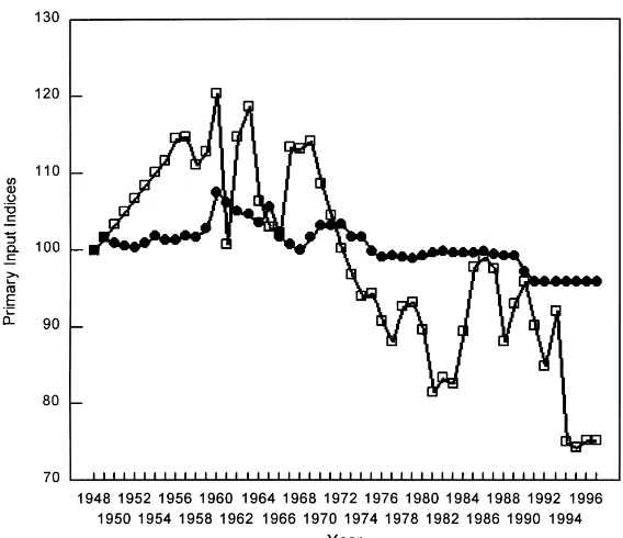
Fig. 3. Divisia input indices for labor and land, for 1948–1997.
intermediate inputs grew at over 5% per annum before 1978 and declined at 0.19% a year since then; capital inputs increased at 2.53% per annum until 1983 and since then have decreased at 3.79% a year.
To better understand these changes, more disag-gregated series are needed which allow the indices to be related to policy changes in the economy. The land index was growing during the period when cultivated area was expanding. Fig. 3 shows that it grew at 0.3% a year through 1960 and then began a slow decline of about 0.25% per annum for the rest of the period. The labor index grew rapidly un-til 1959, at 1.3% per annum, then wavered unun-til the late 1960s, before beginning a decline of 1.18% a year, from 1968 to 1980. During the growth years up to 1970, the cultivated area under maize produc-tion increased in the summer rainfall areas, as oxen were replaced with tractors. Larger areas could be managed and labor use increased, partly due to the spread of fertilizer and high yield varieties. After 1970, the mechanization effect dominated, especially as the combine was introduced and it alleviated the heavy labor demand at harvest time (Sartorius von Bach and van Zyl, 1991). In this respect, the
summer rainfall areas followed the pattern in the winter rain regions, where the expansion of culti-vated area was largely complete by 1947 and the whole period would have been characterized by the substitution of machinery for labor.
Social policies contributed to the decline in em-ployment, including measures restricting the mobility of labor (the Pass Laws), which became severe after 1965. The effects of economic policies were probably greater than social policies, as these included cheap credit, negative real interest rates and tax breaks, al-lowing capital equipment to be written off in the year of purchase. There can be little doubt that these price distortions and policies led to unwarranted substitu-tion of capital for labor, imposing substantial social and economic costs on the rural poor (van Zyl et al., 1987).
D. Schimmelpfennig et al. / Agricultural Economics 23 (2000) 1–15 5
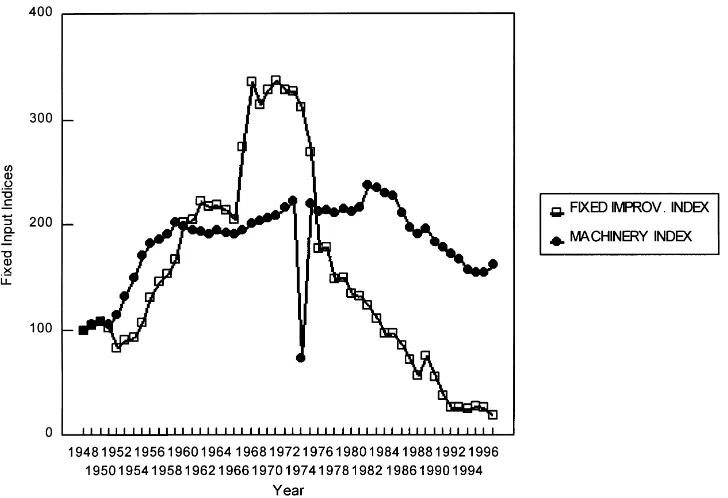
Fig. 4. Divisia capital indices for fixed improvements and machinery, for 1948–1997.
The machinery input index grew at 7.57% a year until 1958; then, at 0.76% per annum until 1981, and has fallen 2.9% a year ever since, partly due to the negative effects of the drought, but in the longer run because of a dramatic change in relative prices. By 1980, economic sanctions protesting apartheid had be-gun to damage the economy and the gold price col-lapsed, forcing the government to devalue the Rand substantially and to end credit subsidies and tax con-cessions on machinery purchases. Thus, the price of imported machinery rose considerably relative to the price of a domestic input like labor and the price dis-tortions which had maximized rural unemployment were ended. Farmers were forced to be more compet-itive and efficient, and at undistorted relative prices, substituted labor for machinery. This accounts for the partial recovery of the labor index in Fig. 3 and the decline in the machinery index in Fig. 4. Fig. 4 also shows the series for buildings and fixed improvements, which falls rapidly from the early 1970s. This is also policy-induced, as the Pass Laws became more severe from 1968 and subsidies for building housing for black workers were withdrawn.
Thus, in the South African case, the policy changes have been so extreme that policy variables explain a considerable proportion of the changes in productivity. We now turn to the effects of the economic variables that account for long-term TFP growth.
2.1. Explaining TFP growth
Changes in the TFP index should be explained by determining variables, such as R&D expenditures. Fol-lowing the literature, and using the Cobb Douglas function, Yt is aggregate output, Xj t are traditional in-puts,2gtare determining variables andβjandγgare parameters. The production function can be written as
Yt =π Xβjj tπ θgtγ g. (1)
Rather than estimating the production function di-rectly, a Tornqvist–Theil index was used to aggregate the outputs Yit and the conventional inputs Xj t. This allows (1) to be written in TFP form, as
Ln(TFP)t = ˆ Y ˆ X
where the aggregate index for the inputs is
which is the logarithm of the ratio of two successive input quantities (the Xj t’s) weighted by a moving av-erage of the share of the input in total cost (the Cj t’s). Since there are multiple outputs, as well as inputs, the same aggregation procedure is applied to give the Tornqvist–Theil output index:
which is the logarithm of the ratio of two successive output quantities weighted by a moving average of the share of the output in total revenue. All the indices reported are chained, so that each value is calculated relative to the previous observation, rather than a base year. The TFP index is simply the ratio of the chained output index and the chained input index.
The Xj’s include all the conventional inputs such as land, labor, capital, machinery, buildings, chemi-cals and other miscellaneous inputs. The2g’s are the stock of accumulated research capital (K), extension expenditures (X), the number of international patents pertaining to agricultural chemicals and machinery (P), the US TFP index (T), and farmer education (E). US TFP is included to cover spillovers of technology from other research jurisdictions. The patent variable includes both private spillovers from abroad and the technology provided by multinational seed, chemical and machinery companies, regardless of whether they are undertaking research in South Africa or not.
Unfortunately, very little is known about R&D in the purely domestic South African private sector, but this need not prevent economic analysis of the returns to R&D, as this is already included in the market system. Indeed, as was noted by Griliches (1979), if agricul-tural inputs were supplied by a monopolist, and input statistics took proper account of quality adjustments, technical change emanating from the private sector input industries would be fully included in the in-put series. Such technological changes are in the farm inputs sector, not the farm sector itself (Kislev and Peterson, 1982), and would not present any difficul-ties. It is only to the extent that the input suppliers are
not monopolists that the statistical sources fail to mea-sure inputs in efficiency units, making it necessary to make some allowance for private R&D expenditures. However, due to these two factors, not all technical change in the input industries is correctly measured at source and there will be some spillover that is still captured in the measures of agricultural productivity. Thus, in estimating the returns to R&D, all the pub-lic expenditures should be included on the cost side as well as a proportion of private expenditures. For Europe and the US, the impact of the private sector may be more pronounced than we assume it is here (Schimmelpfennig and Thirtle, 1999).
Accumulated research capital (KS), can be defined very simply as the sum of past R&D expenditures:
KSt =
X
Rt−i (5)
but if there is no research, there should be negative growth of Kt. For example, in plant breeding, yield gains tend to be lost over time if research on a par-ticular variety is not maintained, as pests and diseases evolve, making the variety susceptible to attack when it was previously immune. Hence, maintenance ex-penditures are required to prevent falling productivity (Blakeslee, 1987).
The alternative to including an arbitrary deprecia-tion factor in the calculadeprecia-tion of KSt is to include a fi-nite number of lagged Rt−i’s as explanatory variables. Initially, the effect of R&D on productivity is expected to be small and then to reach a peak, before diminish-ing to zero as the new technology becomes obsolete. Following this procedure, adding a constant (A) and a stochastic error term gives the customary model
Ln(TFP)t=LnA+XαiLnRt−i+γ1LnXt−i +γ2LnEt−i +γ3LnPt−i+γ4LnTt−i +γ5Wt+Ut (6) where TFPt is the productivity index, Rt−i is R&D lagged i years and all the other variables except the weather have varying lags of i years. Khatri et al. (1998) have established that these variables are Granger prior to TFP. Ut is the remaining stochastic error.
D. Schimmelpfennig et al. / Agricultural Economics 23 (2000) 1–15 7
Fig. 5. Alternative distributed lag effects of research on productivity, for 1948–1997.
Only R&D, extension and education were significant, and the net internal ROR was found to be 64%.2
2.2. Modeling the distributed lags for R&D and patents
The primary focus of the paper is in determining, and using in an ROR calculation, the length and shape of the lag between R&D and TFP. The first stage of the analysis is to determine the length of the lag by estimating an unrestricted finite lag model, with lag length k. Using fewer lags than the true specification implies biased estimates and too many lags implies in-efficient estimates. The lag length is found by search-ing over a range, ussearch-ing appropriate model selection criteria. Geweke and Meese (1981) investigate vari-ous model selection criteria for this purpose, including the Akaike information criterion (AIC), the final pre-diction error (FPE), the Bayesian estimation criterion (BEC) and the Schwartz criterion (SC). The tests are not always in agreement, but for R&D, all the tests confirmed a lag of 9 years.
The second stage involves determining the shape of the lag, and the conventional inverted U-shaped second
2The gross ROR is based on the gross value of output, whereas net RORs are calculated using the value of output minus the value of inputs.
degree polynomial fitted the South African data poorly relative to asymmetric alternatives. Amongst the large number of alternative lag structures tested, general-izations of the exponential and Gamma distributions (Schmidt, 1974) gave the best results according to the model selection criteria.3 Fig. 5 shows the three struc-tures that gave the best results and compares them with the second degree polynomial. The selection criteria clearly reject the second degree polynomial (PDL(2)). Of the other structures, the linear exponent exponen-tial, with a 1-year lead time (EXP(1) LEAD 1) is pre-ferred. The strong negative skew, with a peak in the second year, followed by a decline very much like ge-ometric decay, is very different from the second de-gree polynomial. The early peak has a marked effect on the ROR calculation, which we will show is sensi-tive to the distribution of returns over time.
This result can be contrasted with similar tests for the UK system, where the lag was 16 years and the distribution was positively skewed, with the peak
effects at 12–16 years (Khatri, 1994). This suggests that, whereas the UK system includes a high pro-portion of basic scientific research with a long ges-tation period, the South African research system is dominated by short-term developmental and applied work. This is despite the fact that government-funded research in the universities is included.
Applying the same method to the patent count se-ries gave a lag of 12–13 years and again a negatively skewed exponential distribution. The longer lag on the patent series might be because mechanical innovations are embodied in capital items and the capital stocks adjust slowly. The lags on extension and education should be far shorter than those for R&D, so the same elaborate lag structures are not imposed. Indeed, the model selection criteria indicate that a one-period lag is the appropriate specification.
Incorporating the exponential lag structures in the estimation of Eq. (6) shows how much the lag struc-ture matters. The R&D lag is so precise that none of the other variables except the weather have any ex-planatory power and even the net ROR is an implau-sible 170%. Thus, careful determination of the lag structures has the unfortunate effect of destroying the conventional two-stage model.
2.3. Using the lag structures in the profit function
The poor results from the refined version of the two-stage model suggest that an integrated approach may be preferable. Including the technology variables in the estimation of the residual profit function is less restrictive than the two-stage approach, but the model is too complex and there are insufficient de-grees of freedom to allow much in the way of testing for the best formulation. Thus, the lags and deprecia-tion rates in previous studies have often been chosen somewhat arbitrarily. In this case, prior estimation of the two-stage model provides information on the lag structures of the technology variables, that can be in-corporated in the profit function. Thus, the R&D cap-ital stock is constructed using the perpetual inventory model (PIM), which exhibits the same pattern of ge-ometric decay as the exponential lag. This knowledge stock (KS), with R&D entering with a one-period lag, is then
KSt =RDt+(1−δ)KSt−1 (7)
whereδ is the rate of depreciation. This depreciation rate is set at 10%, so that 90% of the weight is on the first 9 years, the length selected for the exponential lag previously. There is no problem with choosing a starting value for KS because data is available back to 1929, so by 1947, the starting value of KS in 1929 is irrelevant.
The same approach is applied to the other vari-ables, so the patent knowledge stock is approximated in the profit function by a PIM with a depreciation rate of 8.3%, which is appropriate for a 12-year lag. Lastly, extension expenditures and farmer education are included in the model with a simple 1-year lag, as before. Thus, all the information on lag structures gleaned from the two-stage approach are incorporated into the less restrictive integrated model, to which we now turn.
3. The residual profit function model
Assuming that farmers maximize expected prof-its, the normalized restricted profit function (Lau, 1976), with conditioning factors included as fixed inputs, is used to model farmer behavior. Consider a multiple output technology producing outputs Y, (y1, . . . , ym), with the respective expected output prices P, (p1, . . . , pm), using n variable inputs X, (x1, . . . , xn) with prices W, (w1, . . . , wn). Variable expected profits are defined as
π=
The expected prices are taken to be the actual prices from the previous year. This is in accordance with the findings of van Schalkwyk et al. (1994), who con-cluded that naive price expectations explain aggregate South African farmer behavior better than other ex-pectation models.
D. Schimmelpfennig et al. / Agricultural Economics 23 (2000) 1–15 9 of normalized restricted profits, and thus, the
normal-ized expected profit function can be represented as
5∗=5∗
where 5 represents the normalized restricted profit function, Z is the vector of fixed and quasi-fixed inputs, 2 is the vector of technology variables, or conditioning factors (also treated as quasi-fixed in Eq. (9)) and (∗) indicates optimized levels. The the-oretical restrictions on (9) are that the normalized restricted profit function (hereafter called the profit function) is non-decreasing in P, non-increasing in W, linearly homogeneous in prices, twice continuously differentiable and convex in prices, and concave in the quasi-fixed factors (Lau, 1976).
Many studies using time series data employ a time trend as an index of technology. Clark and Young-blood (1992) have demonstrated that the use of a de-terministic time trend with difference stationary pro-duction and price data is inconsistent. By including the (productivity shifting) conditioning factors directly in the objective function, this criticism is addressed in a manner consistent with their recommendations. Quasi-fixed factors (capital stocks) are those that are fixed in the short-run (one production period), but can be varied in the longer run. Fixed inputs and condi-tioning variables, including public and private research expenditures, the international stock of knowledge, ex-tension, farmer education and the weather, are factors of production that cannot be varied by the farmer even in the long run. Thus, profit maximization is assumed to be subject to the levels of these factors.
The functional form employed is the GQ. The GQ profit function is defined as
5=α0+α′Pˆ+δ′2+12Pˆ′βPˆ+122′ϕ2+ ˆP′γ 2 (10)
wherePˆ hat is the stacked vector of normalized out-put and non-numeraire inout-put prices, (P, W)′ and2is the stacked vector of k quasi-fixed, one fixed (for the short-run function) and conditioning factors. The vec-tor α (α1, . . . , αm+n−1) and matrices β (βij, i, j = 1, . . . , m+n−1),φ(φgh, g, h=1, . . . , K+L) andγ (γig, i =1, . . . , m+n−1, g=1, . . . , k+l) contain the parameter coefficients to be estimated. The vector of parametersγ is of particular interest as these are
the shadow prices of the fixed factors and technology variables. Applying Hotelling’s lemma, we derive the (short-run) optimal levels of output supply and input demands:
The long-run profit function differs only in treating all the factors of production as variable inputs. Thus, machinery, land, and the animal capital stocks are assumed to be at their long-run equilibrium levels and there are no quasi-fixed factors. The vector 2 only consists of conditioning factors, such as the weather and technology-related variables, that are al-ways exogenous to the farmer’s decision process. The prices of inputs that were quasi-fixed factors in the short-run model are included in the vector w. Variable input demands for these factors are obtainable using Hotelling’s lemma, and are estimated jointly with other input demands and other supply equations.
The price elasticities are derived as logarithmic derivatives of the supply and derived demand equa-tions with respect to prices. If the elements of 2 are viewed as short-run constraints on production, it is possible to derive the effects of relaxing the2 variable constraints on the output and variable input levels. These fixed factor elasticities are derived as logarithmic derivatives of the supply and derived de-mand equations with respect to the elements of 2 (Lass, 1985; Khatri et al., 1997).
the shadow values of capital, livestock and land can be derived as well as the values for public research, extension, patents and education, which are also cal-culated from the long-run version. The difference be-tween the rental value and the shadow value indicates whether the factor is over, under or optimally utilized. Finally, the shadow value of research can be used to derive the rate of ROR investment (Huffman, 1987).
Dual measures of technological biases can also be obtained from the profit function. Huffman (1987) sug-gests a summary measure which provides input and output biases with respect to the conditioning factors and Khatri (1994) generalizes the conditioning factor biases for a multiple output technology.
4. Data
The national farm-level production data for the pe-riod 1947–1992 were obtained from several sources, largely RSA (1994), and are described in some de-tail in Thirtle et al. (1993). For both the short- and long-run profit function specifications, the three out-put aggregates are crops, horticulture, and livestock and livestock products.
For the short-run profit function, the variable in-puts are Divisia aggregated into four groups: (1) hired labor; (2) machinery running costs (fuel, machinery repairs and other); (3) intermediate inputs (fertilizer, other chemicals, and packing material) and (4) live-stock feed and dips. Vehicles and fixed capital in the form of buildings and other fixed improvements (especially irrigation equipment) are assumed to be quasi-fixed in the short run, as are the stocks of ani-mals. The total area of land in the commercial sector is included as a fixed input.
For the long-run specification, all the conventional inputs are variable. These were Divisia aggregated into the following groups: (1) hired labor; (2) machinery running costs (fuel, machinery repairs and other); (3) intermediate inputs (fertilizer, other chemicals, pack-ing material, feed, and dips); (4) capital, particularly vehicles and other capital in the form of buildings and fixed improvements; (5) livestock and (6) land. The capital stocks are calculated using US depreciation rates (Jorgenson and Yun, 1991, Table 13B, p. 82) in a PIM that assumes geometric decay, as in Ball (1985). The rental prices of the capital stocks are calculated using Jorgenson’s formula to derive long-run capital
service prices from the assumed depreciation rate and the real rate of interest.4
The conditioning factors, that are treated as fixed in-puts in both the short- and long-run specifications, are public research expenditures, public extension expen-ditures, a rainfall index, world patents5 and a farmer education index (ED). The farmer education index is the average number of years of secondary education of farmers, which was kindly provided by the South African Agricultural Union (SAAU).
5. Estimation and results
There are too many parameters in the short-run profit function (10) to estimate the full model in one stage, so the residual profit function approach (Bouchet et al., 1989; Khatri et al., 1997) is used. The system of supply and demand equations, Eqs. (11) and (12), is estimated in the first stage and then the remaining variables are used to explain the residual. The estimated shadow prices and the input biases involve both the parameters from the supply and de-mand system, and the residual profit function. How-ever, as the majority of the parameters for the shadow price and input bias equations are in the supply and demand system, the parameters used in the residual profit function (most of which are significant) can be treated as constants. This allows the derivation of indicative significance bounds for the shadow price and input bias estimates.6
The system of output supply and variable input de-mand equations are estimated for both the short-run and the long-run using the iterative Zellner or seem-ingly unrelated procedure. Each system, with symme-try imposed, produces a set of parameter estimates (not reported here), most of which are significant at the 5% confidence level. The coefficients of determi-nation (R2’s) of the estimated individual supply and demand equations (for both the short-run and long-run
4 We thank Eldon Ball for constructing these series.
5 The patent data comes from the US patent database compiled at the University of Reading by John Cantwell. The series are patent counts, for all agriculture-related chemical and mechanical patents registered in the US.
D. Schimmelpfennig et al. / Agricultural Economics 23 (2000) 1–15 11 specifications) vary between 0.87 and 0.99, which is
high even for time series models. The Durbin–Watson statistics indicate that there are no problems of se-rial correlation in the individual equations. Further, although homogeneity remains a maintained assump-tion (implicitly imposed when normalizing), symme-try and monotonicity, which are necessary conditions for global convexity, are both satisfied by the estimated systems. The estimated profit functions are thus found to be acceptable both with respect to their statistical performance and theoretical consistency.
The results obtained with the short-run and long-run profit functions (that can be estimated in one stage), specifically the elasticity estimates, are in accordance with expectations. The elasticities of the outputs and variable inputs in the long- and short-run estimations are remarkably similar. They are not repeated here as they are almost identical to the short-run profit function results reported by Khatri et al. (1995). As expected, the long-run elasticities for land, cap-ital and livestock are consistently higher than the short-run elasticities. It can therefore be concluded that the results from the short- and long-run models are consistent.
The elasticities show the low supply response of South African agriculture, even over the long run. This result corresponds very closely with the findings of van Zyl (1986) and Sartorius von Bach and van Zyl (1991). It also confirms earlier comments on the abnormal development path of South African agriculture (World Bank, 1994; Kirsten and van Zyl, 1996).
The estimates of the factor-saving biases of techni-cal change show that the Hicks neutrality assumption implicit in the two-stage model is rejected, which is contrary to assumptions implicit in the two-stage ap-proach and may have biased the results. Public R&D has been capital and intermediate input using, and labor and animal input saving. This pattern is typical of developed countries and is hardly appropriate for a country with abundant cheap labor and high rural unemployment. Thus, the public R&D system has exacerbated the damage done by apartheid policies discussed above.
5.1. Shadow prices
Khatri et al. (1998a) established that the shadow price of land is positive, but for livestock, it was not
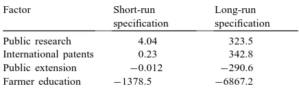
Table 1
Estimated shadow values of the conditioning variables (evaluated at the variable means)a
Factor Short-run
aNote: All the shadow prices are significant at the 0.05 level; shadow values of the short- and long-run conditioning variables are not directly comparable due to differences in the units of measurement of the capital items.
significantly different from zero and for capital it was negative, indicating that policies to reduce capital use could have increased profit. More importantly, they found that the capital stock took 11 years to adjust to changes in input prices. This paper concentrates on the shadow values of the technology variables, which can be interpreted as the marginal change in profits from a unit increment in a technology-related variable. The shadow value for R&D can be used to derive the rate of ROR investment (see Khatri et al., 1996). Note, how-ever, that the shadow values of the short- and long-run conditioning variables are not directly comparable due to differences in the units of measurement of the cap-ital items. These shadow values are reported in Table 1 for both the short- and long-run specifications, eval-uated at the variable means.
In both the short and the long run, public R&D expenditures and international patents have positive and highly significant shadow values, indicating that both the national research system and private sector spill-ins benefit South African agriculture. The two are related in that much of the public research is adaptive in nature and is geared towards exploiting technology that has been developed abroad. The shadow price for public research was negative at the beginning of the period, after which the value rose at an increasing rate, suggesting that the public research system is now making a considerable contribution to profitability (see van Zyl et al., 1993).
expendi-tures were too high. Similarly, the education index ap-pears to have considerable explanatory power in both the short- and long-run formulations, but the shadow price is negative. Since education is a proxy for man-agerial ability, this is contrary to expectations, but this negative result and the weak contribution of extension expenditures are probably related.
The shadow value of education was positive until the early 1960s, but has become increasingly nega-tive since then, and the shadow price of extension has been falling over the period, which suggests that South African commercial farmers have become less depen-dent on public extension advice. This corresponds with the findings of Koch et al. (1991), who show that gov-ernment extension officers spend increasingly more time on administrative duties and do very little ac-tual extension work. Thus, the decline in extension effort could explain the low payoff, but so could re-duced need for extension. The education level of South African commercial farmers is relatively high, so it is entirely possible that the minimum level required to assimilate mass produced research and extension messages has been reached.
But there is a more radical explanation that is far more specific to South Africa. The unreported fixed factor elasticities show that all the input and output elasticities with respect to education are positive, and all but one are highly significant. Thus, education aug-ments output but it also augaug-ments input use, more than proportionately in the case of non-labor inputs. As crop production expanded into climatically marginal and more risky areas, intermediate input use and mech-anization increased considerably in the period from 1965 to the early 1980s (van Zyl et al., 1995). There was evidence of over-mechanization (van Zyl et al., 1987) and fertilizer was often applied (on extension service advice) up to levels where it actually decreased output (Korentajer et al., 1989). This was especially disastrous in the bad climatic conditions of the early and late 1980s (van Rensburg and Groenewald, 1987). Sartorius von Bach et al. (1992) clearly show that it was the better educated farmers who adopted these practices to a greater extent. Thus, educated farmers did respond more strongly to extension service ad-vice, but because maximum physical production (as opposed to maximizing profit) was the major goal and focus of the agricultural research and extension system, the effects were negative.
5.2. Internal rate of return
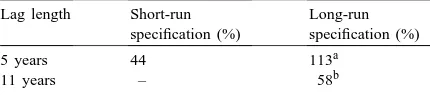
The shadow prices reported above are hard to inter-pret because the technology variables have no obvious prices, and thus, there is no way to compare whether there has been over or under investment. Therefore, the effectiveness of public R&D expenditures can be better interpreted by calculating rates of return (ROR). The shadow values represent the imputed marginal value of a unit increase in knowledge stocks. Thus, to estimate the marginal internal rate of return (MIRR) to research, the additional flow of research investment required to change current knowledge stocks by one unit must be calculated and this will depend on the length and shape of the lag. The MIRR will vary with the choice of the number of periods over which the in-cremental research is distributed. Research is found to affect productivity for 9 years, so the MIRRs reported in Table 2 are for this period of incremental research investments (resulting in a unit change in the knowl-edge stock). The rate of interest that equates this in-cremental research expenditure to the shadow price is the MIRR (Ito, 1991).
The net (output value minus input costs) ROR for the short-run profit function is 44%, while the long-run result is 113%. The lower value is perhaps reasonable for a research system that is to some extent free-riding on the investments made by others. The long-run re-sult is not as high as for the two-stage model, but it is 2.6 times the short-run result. The return will be higher because of the effects of new technology embodied in new capital equipment. Thus, the difference between the two results should depend on the fact that the cap-ital stocks are allowed to adjust in the long-run case. This raises a new problem, since Khatri et al. (1995) found that the capital stock adjusted to changes in the real rate of interest with a long lag of 11 years. The
Table 2
aLag length appropriate for variable long-run inputs (see dis-cussion in Section 5.2).
D. Schimmelpfennig et al. / Agricultural Economics 23 (2000) 1–15 13 12–13-year lag for the patent series, reported above,
corroborates this period of adjustment. This suggests that, although the negatively skewed 9-year lag, with a peak effect after 2 years, may be appropriate for the short-run profit function, it is hard to reconcile with long-run adjustments in fixed or quasi-fixed fac-tors. Therefore, the short lag may be appropriate for R&D on variable inputs like seed varieties and agro-nomic improvements, but R&D on capital items like irrigation equipment, cultivation implements and other specialized machinery must take longer than 2 years to have a peak effect. The difference between the short-run and long-run RORs should result from the technology that is embodied in the capital items. If this is so, then the effects will only occur when the capital stock has adjusted.
To take the adjustment period of 11 years into ac-count, without knowing the lag distribution, the MIRR for the long run is calculated with a lag of 11 years be-tween the unit increment in the knowledge stock and the shadow value. This gives the last figure in Table 2, of 58%, which may be a more realistic estimate of the long-run net ROR. These are certainly respectable rates of return on public expenditure, with the usual qualifications that the figures may be somewhat dimin-ished if we adjust for the dead-weight losses associ-ated with tax collection and the possibility that public funding may be crowding out private sector research. Of greater interest is the sensitivity of ROR calcula-tions to assumed lag structure, particularly when the lag in the effect of R&D on TFP is skewed, negatively in this case, so benefits are exposed to less discounting than if the lag structure were to be symmetric.
6. Conclusion
This paper reports TFP calculations for South African commercial agriculture that show the dam-age caused by the policies of the apartheid era, both in terms of low productivity growth and the unwar-ranted substitution of scarce capital for abundant labor. The shadow price of capital is found to be neg-ative, which leads to restructuring problems when it takes the capital stock 11 years to adjust to changes in input prices. This long lag, from the fixed nature of capital investments, is no doubt also related to apartheid policies which are now gone, but still might
imply that over a decade is required to turn around an over-capitalization problem. In fact, since the col-lapse of the Rand with the gold price that occurred in the early 1980s, we would not expect the overcapital-ization to be corrected by the end of the data series used here.
TFP growth is explained by public R&D and ex-tension expenditures, farmer education and spill-ins of private R&D. This two-stage approach allows the lags to be investigated and the lag between public R&D and TFP is found to be only 9 years long, with a strong negative skew, giving a peak effect after only 2 years. This is because of the adaptive focus of the South African research system, and can be compared with an 18-year positively skewed lag for the UK sys-tem, which undertakes far more basic research. This lag shape results in a rate of return to R&D of 170% and has the effect of making all the other variables insignificant.
To improve the results, the lag structures established in the two-stage approach are used in constructing the technology-related variables included in the estimation of short- and long-run residual profit functions. These profit functions conform to theoretical requirements and produce reasonable estimates of the shadow val-ues of the technology-related variables. The short-run net ROR is found to be 44%, but the long-run ROR is not clear. If the short lag is accepted, the ROR is 113%, but if the capital stock adjustment lag is taken into account, the ROR falls to 58%. More generally, the results show that the ROR is critically dependent on the length and especially the shape of the lag. There is also a problem in determining the long-run ROR in any case, where the estimated lag on R&D is less than the adjustment period of the capital stock. This issue has not arisen in studies of the developed countries be-cause the R&D lag for systems that perform substan-tial basic research is far longer than for South Africa, which concentrates on adaptive research. The ques-tion remains how sensitive ROR calculaques-tions might be, even in developed settings, to a significantly skewed distribution of research benefits.
Acknowledgements
the Development Bank of Southern Africa for financial support. The views expressed are those of the authors and do not necessarily represent policies or views of the US Department of Agriculture.
References
Ball, V.E., 1985. Output input and productivity measurement in US agriculture, 1948–79. Am. J. Agric. Econ. 67 (3), 475–486. Blakeslee, L., 1987. Measuring the Requirements and Benefits of Productivity Maintenance Research, in Evaluating Agricultural Research and Productivity, Proceedings of a Symposium, Atlanta, Georgia, Jan 1987, Miscellaneous Publication 52-1987, Agricultural Experiment Station, University of Minnesota, St Paul, MN.
Bouchet, F.C., Orden, D., Norton, G.W., 1989. Sources of growth in French agriculture. Am. J. Agric. Econ. 71 (2).
Clark, J.S., Youngblood, C.E., 1992. Estimated duality models with biased technical change. Am. J. Agric. Econ. 72 (2), 353–360. Diewert, W.E., 1974. Applications of duality theory. In: Intriligator, M.D., Kendrick, D.A. (Eds.), Frontiers of Quantitative Economics, Vol. 2. North-Holland Publishing Company, Amsterdam.
Echeverria, R. (Ed.), 1990. Methods for Diagnosing Research System Constraints and Assessing the Impact of Agricultural Research. ISNAR, The Hague.
Evenson, R.E., Landau, D., Ballou, D., 1987. Agricultural productivity measures for US states. In: Proceedings of a Symposium, Atlanta, GA, 29–30 January 1987, Miscellaneous Publication 52-1987, MN, Agricultural Experiment Station, University of Minnesota, St. Paul, MN.
Geweke, J., Meese, R., 1981. Estimating regression models of finite but unknown order. Int. Econ. Rev. 20, 203–216. Griliches, Z., 1979. Issues in assessing the contribution of R&D
to productivity growth. Bell J. Econ. 10 (1), 92–116. Huffman, W.E., 1987. Research bias effects for input–output
decisions: an application to US cash-grain farms. In: Proceedings of a Symposium, Atlanta, GA, 29–30 January, 1987, Miscellaneous Publication 52-1987, Agricultural Experiment Station, University of Minnesota, St. Paul, MN. Ito, J., 1991. Assessing the Returns of R&D Expenditures on
Post-War Japanese Agricultural Production, Research Paper No. 7, National Research Institute of Agricultural Economics, Ministry of Agriculture, Forestry and Fisheries, Tokyo. Jorgenson, D.W., Yun, K.-Y., 1991. Tax reform and the cost of
Capital. Oxford University Press, New York.
Khatri, Y.J., 1994. Technical change and the returns to research in UK agriculture, 1953–1990. Ph.D. Dissertation, University of Reading, England.
Khatri, Y., Thirtle, C., van Zyl, J., 1995. South African Agricultural Competitiveness: A Profit Function Approach to the Effects of Policies and Technology, pages 670–684, in G.H. Peters and D.D. Hedley, (Eds.), Agricultural Competitiveness: Market Forces and Policy Choice, Dartmouth Publishing Company, Aldershot.
Khatri, Y.J., Thirtle, C., van Zyl, J., 1996. Public research and development as a source of productivity change in South African agriculture. South African J. Sci. 92, 143–150.
Khatri, Y.J., Jayne, T., Thirtle, C., 1997. ‘A Profit Function Approach to the Efficiency Aspect of Land Reform in Zimbabwe’, pp. 77–84 in R. Rose, C. Tanner and M.A. Bellamy (Eds.), Issues in Agricultural Competitiveness, Occasional Paper Number 7, International Association of Agricultural Economists. Published by Dartmouth Publishing Company, Aldershot.
Khatri, Y.J., Thirtle, C., van Zyl, J., 1998. Research and Productivity Growth in South African Agriculture, 1947–91: the Two-Stage Decomposition Approach, Chapter 5 in J. van Zyl and C. Thirtle (Eds.), Productivity, Efficiency and Land Markets in South African Agriculture, HSRC Printers, Pretoria. Khatri, Y.J., Thirtle, C., van Zyl, J., 1988a. Sources of Productivity Growth in South African Commercial Agriculture, 1947–91: A Profit Function Approach, Chapter 4 in J. van Zyl and C. Thirtle (Eds.), Productivity, Efficiency and Land Markets in South African Agriculture, HSRC Printers, Pretoria.
Kirsten, J.F., van Zyl, J., 1996. The contemporary policy environment: undoing the legacy of the past. In: van Zyl, J., Kirsten, J.F., Binswanger, H.P. (Eds.), Policies, Markets and Mechanisms for Agricultural Land Reform in South Africa. Oxford University Press, Cape Town.
Kislev, Y., Peterson, W.L., 1982. Prices, technology and farm size. J. Polit. Econ. 90, 578–595.
Koch, B.H., van Zyl, J., van der Wateren, J.J., 1991. The role of extension in the development of the farmer as entrepreneur. Develop. Southern Africa 8 (1), 127–136.
Korentajer, L., Berliner, P.R., Dijkhuis, F.J., van Zyl, J., 1989. Use of climatic data for estimating nitrogen fertilizer requirements of dryland wheat. J. Agric. Sci. 113, 131–137.
Lass, D.A., 1985. Estimation of total factor productivity growth in the corn belt region: a dual approach to measurement. Ph.D. Thesis, Pennsylvania State University, PA.
Lau, L.J., 1976. A characterization of the normalized restricted profit function. J. Econ. Theory 12(1).
RSA, 1994. Abstract of Agricultural Statistics 1994. Directorate of Agricultural Economic Trends, Department of Agriculture, Pretoria, South Africa.
Sartorius von Bach, H.J., van Zyl, J., 1991. Have recent structural changes caused agriculture to become less rigid? Develop. Southern Africa 8 (3), 399–404.
Sartorius von Bach, H.J., van Zyl, J., Koch, B.H., 1992. Managerial ability and problem perceptions: a case study of economic survival and failure in mixed dryland farming. South African J. Agric. Extension 22, 13–18.
Schimmelpfennig, D.E., Thirtle, C., 1999. The internationalization of agricultural technology: patents, R&D spillovers and their effects on productivity in the European Union and United States. Contemporary Econ. Policy 17 (4), 457–468.
Schmidt, P., 1974. An argument for the usefulness of the gamma distributed lag model. Int. Econ. Rev. 15, 246–250.
D. Schimmelpfennig et al. / Agricultural Economics 23 (2000) 1–15 15 Thirtle, C., Sartorius von Bach, H., van Zyl, J., 1993. Total
factor productivity in South African agriculture, 1947–91. Develop. Southern Africa 10 (3), 301–317.
Thirtle, C., van Zyl, J., 1994. Explaining TFP growth in South Africa: the returns to R&D and extension. South African J. Agric. Extension. 23.
van Rensburg, B.J., Groenewald, J.A., 1987. The distribution of financial results and financial ratios among farmers during a period of financial setbacks: grain farmers in Western Transvaal, 1981/82. Agrekon 26(1).
van Schalkwyk, H.D., van Zyl, J., van Rooyen, C.J., Kirsten, J.F., 1994. The agricultural land market in South Africa: options for land reform. Paper presented at the 21st IAAE International Conference, Harare, Zimbabwe, August 1994.
van Zyl, J., 1986. Duality and elasticities of substitution: theoretical considerations and an empirical application. Develop. Southern Africa 4 (1), 65–73.
van Zyl, J., Fényes, T.I., Vink, N., 1987. Labor-related structural trends in South African maize production. Agric. Econ. 1 (3), 241–258.
van Zyl, J., McKenzie, C.C., Kirsten, J.F., 1995. Natural resource issues in rural South Africa. In: van Zyl, J., Kirsten, J.F., Binswanger, H.P. (Eds.), Policies, Markets and Mechanisms for Agricultural Land Reform in South Africa. Oxford University Press, Cape Town.
van Zyl, J., van Schalkwyk, H.D., Thirtle, C., 1993. Entrepreneurship and the bottom line: how much of agriculture’s profits is due to changes in price, how much to productivity? Agrekon 32 (4), 223–229.