An analytical model for estimating canopy transpiration and carbon
assimilation fluxes based on canopy light-use efficiency
M.C. Anderson
a,∗, J.M. Norman
a, T.P. Meyers
b, G.R. Diak
caDepartment of Soil Science, University of Wisconsin-Madison, 1525 Observatory Drive, Madison, WI 53706, USA bNOAA/ATDD, 456 South Illinois Avenue, Oak Ridge, TN 37830, USA
cCooperative Institute for Meteorological Satellite Studies, University of Wisconsin-Madison, 1225 West Dayton Street, Madison, WI 53706, USA
Received 29 March 1999; received in revised form 28 October 1999; accepted 9 December 1999
Abstract
We develop a simple, analytical model for canopy resistance to canopy–atmosphere gas exchange that is well suited for incorporation into regional-scale land-surface parameterizations. This model exploits the conservative nature of canopy light-use efficiency (LUE) in carbon assimilation that is observed within broad categories of plant species. The model paradigm assumes that under standard environmental conditions, a canopy will operate at the field-measured LUE, but will deviate from this standard efficiency as conditions change. Effective LUE estimates generated by the model respond to variations in atmospheric humidity, CO2concentration, the composition of solar irradiation (direct versus diffuse beam fractions), and soil
moisture content. This modeling approach differs from scaled-leaf parameterizations in that a single estimate of nominal canopy LUE replaces both a detailed mechanistic description of leaf-level photosynthetic processes and the scaling of these processes from the leaf to canopy level. This results in a model that can be evaluated analytically, and is thus computationally efficient and requires few species-specific parameters. Both qualities lend themselves well to regional-and global-scale modeling efforts. For purposes of testing, this canopy resistance submodel has been embedded in the Atmosphere–Land Exchange (ALEX) surface energy balance model. The integrated model generates transpiration and carbon assimilation fluxes that compare well with estimates from iterative mechanistic photosynthetic models, and with flux measurements made in stands of corn, soybean, prairie grasses, desert shrubs, rangeland, and black spruce. Comparisons between modeled and measured evapotranspiration (LE) and carbon assimilation (Ac) fluxes yield mean-absolute-percent-differences of 24% (LE) and 33% (Ac) for hourly daytime fluxes, and 12% (LE) and 18% (Ac) for daily-integrated fluxes. These comparisons demonstrate robustness over a
variety of vegetative and climatic regimes, suggesting that this simple analytical model of canopy resistance will be useful in regional-scale flux evaluations. ©2000 Elsevier Science B.V. All rights reserved.
Keywords:Canopy; Carbon assimilation; Evapotranspiration; Light-use efficiency; ALEX
∗Corresponding author. Tel.:+1-608-265-3288;
fax:+1-608-265-2595.
E-mail address:[email protected] (M.C. Anderson).
1. Introduction
Stomata simultaneously regulate both the influx of carbon dioxide and the efflux of water between a leaf and its environment, constantly modifying the resistance to gas exchange in response to changing environmental conditions to maintain plant growth
while minimizing water loss. On the scale of the individual leaf, the relevant regulating quantity is the stomatal resistance (Rst), which depends on the
distribution and condition of stomata on the leaf sur-face. Landscape-level fluxes scale inversely with the canopy resistance (Rc), representing the bulk stomatal
resistance to gas exchange exerted by all leaves in the canopy in aggregate. The canopy resistance therefore provides a key for predicting both carbon assimila-tion and transpiraassimila-tion fluxes from vegetated surfaces. The predictive power of many climate and mesoscale forecast models has been significantly enhanced by the incorporation of a simple representation ofRcinto
the model land-surface parameterization (Avissar and Pielke, 1991; Dickinson et al., 1991; Mascart et al., 1991; Randall et al., 1996).
Canopy resistance is often estimated by applying detailed mechanistic models of photosynthesis-stomatal response developed for individual leaves (e.g., Col-latz et al., 1991, 1992), then scaling leaf responses to the canopy level using models of light penetration and leaf adaptation as functions of position within the canopy (e.g., Sellers et al., 1996). While this bottom-up scaling approach has proven effective in reproducing observed assimilation fluxes, it involves the specification of many species-dependent parame-ters and requires a computationally expensive iterative solution that can become numerically unstable under certain conditions (Baldocchi, 1994). The accuracy of such an approach depends on the validity and ro-bustness of the assumed scaling principles, which are strongly non-linear (see review by Norman, 1993).
An alternative is to model the canopy response to its environment in bulk, neglecting the behavior of in-dividual leaves. For many applications, there are com-pelling reasons to approach the problem in this way. McNaughton and Jarvis (1991) demonstrate that neg-ative feedbacks develop within the canopy system that can cause the canopy to have a more stable behavior in the face of environmental fluctuations than would an isolated leaf. They show that transpiration rates be-come less sensitive to changes in atmospheric tem-perature and vapor pressure deficit (VPD) and more tightly coupled to incident light as scale increases from the leaf to canopy level. Canopy carbon assimi-lation rates also respond more conservatively (and lin-early) to modifying factors in comparison with rates observed in individual leaves (Haxeltine and
Pren-tice, 1996). Therefore, detailed models of stomatal response often may not provide additional accuracy in estimating stand-level fluxes. Furthermore, simple scaling techniques may neglect important feedback and system effects.
Here, we propose an approach to modeling canopy resistance that exploits the conservative nature of tran-spiration and photosynthetic processes occurring on the stand level. The fundamental quantity used in this technique is the canopy light-use efficiency (LUE, des-ignatedβ), defined here as the ratio between the net canopy carbon assimilation rate (Ac) and the photo-synthetically active radiation (PAR) absorbed by the canopy (APAR). LUE has been measured for many different plant species, and has been found to be fairly conservative within vegetation classes when the plants are unstressed. Because assimilation scaling effects are implicitly incorporated into stand-level measure-ments of LUE,βcan provide a valuable constraint to canopy resistance modeling.
β-constrained models are particularly well-suited to application over large geographical regions because they are founded on a quantity that can be derived with reasonable accuracy from remote sensing: APAR (e.g., Kumar and Monteith, 1981; Daughtry et al., 1983; Steinmetz et al., 1990; Myneni et al., 1995a, b; Landsberg et al., 1997). β models typically require fewer equations, fewer tunable-parameter specifica-tions, and fewer ground-based measurements than do scaled-leaf parameterizations. For these reasons, many recent models of global net primary production have been constructed upon principles of LUE (e.g., Potter et al., 1993; Ruimy et al., 1994; Prince and Goward, 1995).
Here we derive a simple, analytical expression for canopy resistance that is semi-constrained by field measurements of canopy LUE, averaged over broad vegetation categories. Despite its simplicity, this equation reproduces many of the subtle dependencies of LUE on environmental factors that are observed in nature. When embedded within the framework of a two-source (plant+soil) model of Atmosphere-Land Exchange (ALEX1), this equation provides hourly and daily estimates of evapotranspiration and carbon assimilation fluxes that agree well with microme-teorological measurements made in stands of corn,
soybean, prairie grasses, desert shrubs, rangeland, and black spruce.
2. Light-use efficiency
Numerous studies have demonstrated linearity in the relationship between the increase in canopy biomass during vegetative growth and the amount of visible light intercepted or absorbed by leaves in the canopy (Monteith, 1966, 1972; Puckridge and Don-ald, 1967; Duncan, 1971). Linear relationships are also observed between photosynthetic carbon uptake and radiation receipt by a canopy. While this relation-ship can be markedly non-linear for individual leaves, curvature decreases on the canopy level, presumably because a smaller fraction of leaf area is operating under light-saturated conditions (Hesketh and Baker, 1969). Haxeltine and Prentice (1996) demonstrate that the semi-mechanistic photosynthesis models of Col-latz et al. (1991, 1992) will yield linear relationships between assimilation and light interception when in-tegrated over the canopy if it is assumed that the canopy redistributes nitrogen content to achieve opti-mal photosynthetic functioning. Furthermore, there is some evidence to suggest that the slope of this linear relationship, the canopy LUE, may be fairly conser-vative within the major vegetation classes, perhaps as a result of natural selection (Field, 1991; Goetz and Prince, 1998a). This is intriguing, because conser-vative relationships in nature often facilitate simpler modeling strategies.
The conservative nature of LUE in carbon uptake, however, is sometimes difficult to ascertain from the literature due to the wide variety of definitions and measurement techniques that have been employed in different experiments (see discussion in Norman and Arkebauer, 1991; Gower et al., 1999). In brief, the difficulties arise because these experiments have not adopted a common definition of (a) ‘light use’ nor of (b) ‘carbon uptake’. A definition of light use requires identifying a bandwidth (total solar versus PAR), a form of usage (absorption versus interception), and a medium for utilization (green versus living and dead vegetation; leaves, stems, branches, flowers or whole plant). Carbon uptake has alternately been defined as carbon fixed by photosynthesis (assimilation) or as biomass increment (above ground, or above+below
ground). Often subtle mechanisms for biomass losses, such as herbivory, decomposition, and root slough-ing, have been disregarded. Finally, an appropriate interpretation of light-use and carbon-uptake mea-surements depends on the measurement time and timescale (hour, day, day+night, season). For exam-ple, daytime measurements of LUE exclude night respiration costs and will thus overestimate multi-day averages.
For the purposes of studying net primary production in terrestrial ecosystems, Gower et al. (1999) com-piled from the literature a list of LUE measurements based on annual or seasonal biomass accumulation for several major vegetation types and converted them to a common unit of grams total (above+below ground) net primary production per MJ APAR. APAR is the preferable definition of light use in this context be-cause (a) photons in the PAR band are most intimately involved in the photosynthetic process, while NIR pho-tons in the solar spectrum are predominantly reflected or scattered by the canopy; and (b) the fraction of in-cident PAR absorbed by green vegetation (fAPAR) is
a quantity that can be remotely sensed as has been shown with both empirical (e.g., Daughtry et al., 1983; Steinmetz et al., 1990; Landsberg et al., 1997) and theoretical studies (e.g., Kumar and Monteith, 1981; Myneni et al., 1995a, b). Gower et al. (1999) pre-scribe the conversion process for different definitions of light use and carbon uptake used in the original papers.
For our purposes here, focussing on fluxes rather than productivity, we define LUE as ‘the net carbon dioxide uptake by the canopy (intake less respiration, in moles) per mole PAR photons absorbed by green vegetation in the canopy.’ Productivity estimates can be extracted if the conversion from moles carbon se-questered to grams dry matter is known. This con-version efficiency is species-specific and depends on the amount of carbon required to build carbohydrates, proteins and lipids and the relative amounts of these constituents within the plant tissues. Vertregt and Pen-ning de Vries (1987) tabulate ‘reciprocal glucose val-ues’ (GVI) for describing the energy content of dry matter for several different crops, and Griffin (1994) summarizes construction costs for several tree species.
Conversion from LUE in g NPP (MJ APAR)−1 to
LUE in mol CO2(mol APAR)−1then is accomplished
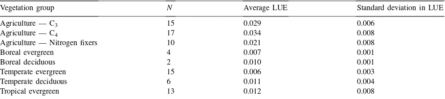
Table 1
Mean and standard deviations among measurements of LUE reported by Gower et al. (1999) for several major vegetation groupsa
Vegetation group N Average LUE Standard deviation in LUE
Agriculture — C3 15 0.029 0.006
Agriculture — C4 17 0.034 0.008
Agriculture — Nitrogen fixers 10 0.021 0.008
Boreal evergreen 4 0.007 0.001
Boreal deciduous 2 0.010 0.001
Temperate evergreen 15 0.006 0.003
Temperate deciduous 6 0.011 0.004
Tropical evergreen 13 0.012 0.008
aAll LUE values have been converted to units of mol CO2mol−1 APAR from their original units of g NPP per MJ APAR using glucose content values from Vertregt and Penning de Vries (1987) and Griffin (1994).Nindicates the number of LUE measurements used to compute the average and standard deviation for each vegetation group.
LUE
Table 1 lists mean values and standard deviations of standardized LUE measurements reported by Gower et al. (1999) for several different vegetation groups, converted into units of mol CO2(mol APAR)-1using
Eq. (1) (the grassland measurements in Gower et al. (1999) have been omitted here because information on light interception was not included in the original pa-pers). When brought to a common standard, the con-servative quality of LUE becomes more apparent (see also Fig. 6 of Gower et al., 1999).
Conservation of LUE is observed most prominently over an annual timescale. Over shorter timescales, there are several factors that will cause temporal vari-ations in LUE. Seasonal cycles in the respiration to as-similation ratio for a given vegetation type will induce synchronized oscillations in net LUE. Evergreens, for example, spend a fraction of the year dormant while still collecting light; LUEs based on annual biomass accumulation will therefore underestimate production during peak growth periods. Because of variability in respiratory behavior between plant species, it is likely that gross LUE (reflecting gross CO2 uptake), and
not net LUE, is the truly conservative quantity (Goetz and Prince, 1998b). Gross LUE, however, is a diffi-cult quantity to measure in practice, and respiration models are still required to infer NPP.
On still shorter timescales (daily and hourly), LUE can be influenced by an array of environmental factors, including extreme temperatures, soil moisture stress, nutrient limitations and high atmospheric VPDs (Run-yon et al., 1994; Landsberg and Hingston, 1996). The variable partitioning of PAR incident above the canopy into direct beam and diffuse components (due to sun angle, clouds, etc.) can also affect LUE (Norman and Arkebauer, 1991). Diffuse light is more evenly dis-tributed over leaves in the canopy, causing a smaller fraction of the leaves to operate in a light-saturated mode where photons are wasted. Carbon uptake effi-ciency in some conifers is particularly sensitive to dif-fuse lighting conditions, as needle photosynthesis can saturate at low quantum flux densities (Leverenz and Jarvis, 1979).
The LUE model as presented here responds to changes in light composition, soil moisture avail-ability, ambient CO2 concentration, and atmospheric
demand; empirical temperature and nutrient response functions will be incorporated in future studies.
3. Model description
3.1. Analytical canopy resistance submodel
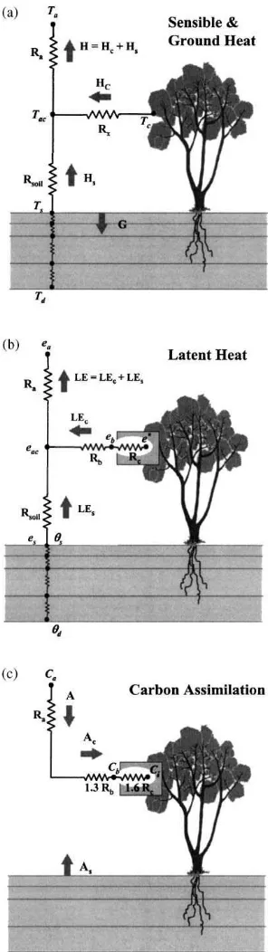
Fig. 1. Transport resistance networks used in the ALEX model to compute fluxes of (a) sensible and soil heating, (b) latent heating and (c) assimilated carbon.
in Appendix A; here we concentrate on the embed-ded analytical submodel for canopy resistance. In the following, the subscripts ‘a’, ‘ac’, ‘b’, and ‘i’ will re-fer, respectively, to bulk average conditions above the canopy, within the canopy air space, within the bound-ary layer at the leaf surface, and inside substomatal cavities (see Fig. 1). The subscript ‘c’ refers to fluxes and properties associated with the canopy in bulk, and ‘s’ to conditions at the soil surface. Model state vari-ables of temperature, vapor pressure, and carbon diox-ide concentration are designated asT(K),e(kPa), and C(mol CO2mol−1air), respectively.
The series–parallel resistance network used in Fig. 1 to define sensible and latent heating establishes feed-back between soil and canopy fluxes and the in-canopy microclimate. Pathways for carbon transport from the soil and vegetation have been decoupled for compu-tational simplicity; this is a reasonable approximation in most circumstances. Note that humidity and carbon concentration conditions at the leaf surface, within the laminar boundary layer, are modeled explicitly in this submodel; these layers can play an important role in mediating feedback loops that influence stomatal response on the canopy level (Collatz et al., 1991; McNaughton and Jarvis, 1991).
In Fig. 1, Rc and Rb are, respectively, the effec-tive stomatal and boundary layer resistances to water vapor diffusion exerted by all leaves in the canopy in bulk,Ra is the aerodynamic resistance to turbulent
transport between the canopy and the measurement reference height, andRs is the resistance through the
boundary layer above the soil surface. Rb is related
toRx, the total two-sided leaf boundary layer
resis-tance integrated over all leaves in the canopy, asRb= (fs/[fg×fdry])Rx. The factorfsadjusts for a possible
inequality in the distribution of stomata over the top and bottom sides of the leaf (fs=1 for amphistomatous
leaves, and 2 for hypostomatous leaves), the fraction of green vegetation in the canopy (fg) excludes stomata on dead leaves from the net transport path, while the dry vegetation fraction (fdry) excludes stomata blocked by liquid water on leaf surfaces, accumulated through precipitation or condensation (evaporative fluxes from the wet leaf area are treated in Appendix A). Forms used here forRa,RxandRsare summarized by Kustas
et al. (2000).
positive away from the canopy in units of W m−2)
and net carbon assimilation (Ac, positive toward the
canopy in units ofmmol m−2s−1) can be written:
whereλis the latent heat of vaporization in Jmmol−1, Pis the atmospheric pressure in kPa, and resistances are in units of m2smmol−1. The air within the stomatal
pores is assumed to be saturated at the mean temper-ature of the canopy,Tc, soei=e*(Tc) and the relative
humidity inside the leaf boundary layer RHb=eb/ei.
The resistance multipliers in the denominators of Eqs. (4) and (5) account for the relative diffusivities of CO2
and water vapor.
Studies of gas exchange with isolated leaves sub-jected to varying environmental conditions have generated a family of simple empirical relationships between stomatal conductance and conditions at the leaf surface. Ball et al. (1987), for example, proposed the linear response function
ments made at the leaf-level. The coefficients b and mhave been measured for several plant species and have been found to be fairly conservative within the C3and C4functional categories (Ball, 1988; Norman
and Polley, 1989; Leuning, 1990; Collatz et al., 1991; Lloyd, 1991; Gutschick, 1996). A scaling from leaf to canopy level is effected by integrating in parallel over all dry, green leaf area (Fdg):
leaf area index. The factor Fdg appears explicitly in
the first term in Eq. (7) and implicitly in the second term in the bulk canopy values ofAc,RHbandCb.
It should be noted that many modified forms of the original Ball et al. (1987) stomatal response function (Eq. (6)) have appeared in the literature since its intro-duction (e.g., Leuning, 1990, 1995; Lloyd, 1991; Kus-tas et al., 2000). These modifications address some of the shortcomings of Eq. (6), including breakdown at very low light, humidity, and CO2levels. Furthermore,
there is evidence to suggest that the primary variable driving stomatal response to humidity is notRHb, but rather saturation VPD (Aphalo and Jarvis, 1991) or transpiration rate (Friend, 1991; Mott and Parkhurst, 1991; Monteith, 1995). Despite these objections, the very simple, linear form in Eq. (6) has proven reason-ably effective over a range of environmental condi-tions. It is used here to minimize the number of tun-able parameters required by ALEX and to facilitate an analytical solution for canopy resistance.
Given measurements or estimates ofF,fg,fdry,Ca, Rb,Ra,eac, andei=e*(Tc) (in this case,eac,Tcandfdry,
are provided by the ALEX model, as described fur-ther), the unknowns in Eqs. (2)–(5) and (7) areRc,Ac, LEc,Cb,Ci, andRHb. One more equation is required
to close the system, and this equation must introduce the dependence of canopy resistance on the incident quantum flux density. Here we invoke the empirical observation that, in the absence of stress conditions, the rate of carbon assimilation by a canopy is nearly linearly proportional to the flux of photosynthetically active radiation absorbed by living vegetation in the canopy (APAR):
Ac=βAPAR (8)
whereβ(mol CO2mol−1quanta) is the canopy LUE.
Under optimal conditions, LUE is found to be rela-tively consistent across plant species within the C3and
C4 classes (see Table 1); however, as discussed
ear-lier, canopy LUE will deviate from this nominal value in response to certain varying environmental condi-tions. To accommodate such modulating effects on as-similation rate,β has been cast as a function of the ratio of intercellular to ambient CO2 concentrations
(γ=Ci/Ca):
Ac=β(γ )APAR. (9)
The concentration of CO2 within the substomatal
cavities,Ci, is regulated by the relative rates of carbon
photosynthetic process. Several studies have shown that γ is remarkably constant for leaves of a given species over a wide range of conditions, with typical values of 0.4 for C4plants and 0.6–0.8 for C3plants
(Wong et al., 1979; Long and Hutchin, 1991). Con-ditions that cause this ratio to vary often affect the canopy LUE as well. For example, stomatal closure in response to a desiccating environment will tend to move the canopy toward a lower value of LUE, while simultaneously decreasing the average Ci through continuing fixation. An enhancement in the ratio of diffuse to direct-beam radiation (i.e., due to low sun angle or increased cloud cover) may increase both LUE andCi, as photosynthetic light-use in the
upper-most leaves in the canopy becomes unsaturated. In general, a positive relationship between,β andCi is
expected on a canopy level.
We assume that under unstressed conditions the canopy will tend to operate near a nominal LUE (βn) with a nominal value of Ci/Ca (γn), both
val-ues being characteristic of the particular vegetation species. Although the functional dependence of Ac
onCi is curvilinear for individual leaves, simulations with the Cupid soil–plant–atmosphere model (Nor-man and Arkebauer, 1991) indicate the relationship becomes linearized on the canopy level. To facilitate a low-order analytical solution forRc, we assume this relationship is approximately linear in the regime that most canopies will tend to operate:
β(γ )= βn
γn−γ0
(γ −γ0). (10)
Typical values for the parameters βn, γn andγ0
for C3and C4canopies have been determined through
numerical experimentation with the Cupid model as-suming an ambient CO2concentration of 340 ppm (see
Table 2). For C4plants, the offsetγ0appears
negligi-ble; however, a significant positive offset is associated with C3canopies. These findings are consistent with
the behavior of the CO2compensation points observed
in C3and C4species (Collatz et al., 1991, 1992).
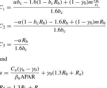
Eqs. (2)–(10) can be combined to yield a cubic function inRc:
Rc3+C1Rc2+C2Rc+C3=0 (11)
where
C1 =
αbc−1.6(1−bcRb)+(1−γ0)meeaci
1.6bc C2=
−α(1−bcRb)−1.6Rb+(1−γ0)mRb 1.6bc
C3=−αRb
1.6bc
and
α= Ca(γn−γ0)
βnAPAR
+γ0(1.3Rb+Ra) R2=1.3Rb+Ra.
The roots of Eq. (11) can be extracted analytically (see, e.g. Press et al., 1992); the positive root corresponds to a physical value for the canopy resistance. Given this estimate ofRc, canopy transpiration can be computed
from Eq. (2), and assimilation by eliminatingCifrom
Eqs. (4) and (9):
Ac= CaβnAPAR(1−γ0)
Ca(γn−γ0)+βnAPAR(1.6Rc+1.3Rb+Ra) .
(12)
The modeled canopy resistance in Eq. (11) responds to changes in light, humidity, CO2concentration, and
moderate variations in leaf temperature (by modu-lating the substomatal saturation vapor pressure,ei). Stomatal closure in response to water stress and ex-treme temperatures can be simulated through incorpo-ration of empirical stress functions (see Section 3.4).
3.2. LUE response to diffuse light fraction
As discussed in Section 2, LUE is known to in-crease under more diffuse lighting conditions, where light is more uniformly and efficiently distributed over the canopy. Norman and Arkebauer (1991) modeled this phenomenon using the Cupid model and found a nearly linear response of LUE to the fraction of PAR that is diffuse (fdif). If 50% beam radiation is used as a reference, instantaneous values of the LUE for corn (C4) may be 15% higher for diffuse light and 15%
lower for a clear sky; however, for soybean (C3), the
variation may be ±40%. The difference in slope is due to the fact that C3canopies saturate at lower light
To capture this response in hourly assimilation es-timates, it is possible to modify the nominal LUE,βn
in Eq. (10) according to
βn′=βn×[1+21dif(fdif−0.5)] (13)
where1dif=0.4 for C3plants and1dif=0.15 for C4.
If only daily-integrated fluxes are of interest,βn can
be left unmodified.
3.3. Temporal considerations — nighttime and seasonal fluxes
The appropriate averaging timescale for evaluating carbon flux estimates using Eq. (11) will depend on the timescale over which the LUE factor was measured. Flux estimates will be most accurate when the averag-ing and measurement timescales are commensurate.
If βn was derived from daytime measurements of Acversus APAR during a particular growth stage, Eq.
(11) should provide reasonable hourly daytime flux estimates for that same growth stage. In this case, nighttime respiration flux can be estimated with an empirical function of canopy temperature.
Ifβn was derived from seasonal dry matter
accu-mulation measurements, Eq. (11) will give good esti-mates of seasonal NPP, but will underestimate daytime fluxes because nighttime respiration costs have been rolled into the LUE measurement. The degree of un-derestimation will depend on the ratio of respiration to net assimilation for each particular plant species. For black spruce, autotrophic respiration is approximately 60–70% of the gross primary production on an an-nual basis (Ryan et al., 1997), so the bias in this case would be large. With NPP-based LUE measurements, it is appropriate to set nighttime values of modeled Ac to zero, so that seasonally-integrated carbon flux
estimates will be unbiased. With a seasonal and/or daily model of the respiration to assimilation ratio, it should be possible to unfold the nighttime respiration costs fromβnand obtain less biased estimates of net assimilation on shorter timescales.
3.4. Stress modification of canopy resistance
The fluxes LEct andAc should be considered the
potential fluxes that the canopy could attain in the absence of vegetative stress. Limiting plant-available
water (‘aw’), nutrients (‘n’), or extreme temperatures (‘t’) can induce stomatal closure and reduce canopy fluxes below these potential levels. Following Jarvis (1976), stomatal response to stress on the canopy level is captured in ALEX through imposition of indepen-dent stress functionals:
Rc′=Rc×faw×ft×fn× · · · (14)
where Rc′ and Rc are stressed and unstressed
(from Eq. (11)) estimates of canopy resistance, respectively.
Studies investigating stomatal response to changes in various water status indicators typically show that stomatal conductance remains at a maximum (po-tential) level until the indicator drops below some threshold, at which point conductance decreases rapidly toward zero. Often the indicator used is leaf water potential, but a direct response to soil water potential has also been demonstrated (Gollan et al., 1986). A soil-water-based stress functional affords a much simpler overall modeling strategy, because leaf water potential depends on both soil moisture status and atmospheric demand.
Campbell and Norman (1998) outline a simple supply/demand-based scheme that relates depletion of the fraction of plant-available water in the root zone:
Aw=
θ−θpwp θfc−θpwp
(15)
to reductions in transpiration due to stomatal closure:
faw=1−23
h
Aw
0.03−1/bs−1.5−1/bs+1.5−1/bsi−bs
(16)
whereθ, θfc, θpwp are, respectively, the actual
vol-umetric soil water content, and the water contents at field capacity and permanent wilting, and bs is
the exponent in the soil moisture release curve. Soil-water-limited transpiration and assimilation rates can then be approximated as
LE′ct =faw×LEct (17)
Ac′=faw×Ac (18)
where the potential fluxes LEct and Ac have been
photosynthesize at nearly their potential rate until they have extracted about half the available water from the root zone; further extraction takes an increasing toll on these exchanges.
Several generic temperature response functions are available in the literature; frequently, simply specify-ing species-dependent upper and lower temperature cutoffs for photosynthetic uptake is sufficient. The effects of extreme temperatures are neglected in the simulation studies presented below because the modeled canopy temperatures were typically within ranges considered optimal for photosynthesis.
3.5. ALEX: A coupled canopy resistance–energy balance model
The field measurements required by the canopy re-sistance submodel described in Section 3.1 are min-imal: above-canopy wind speed (for Ra andRb) and
CO2 concentration (Ca), canopy leaf area index (F)
and fraction of green vegetation (fg), approximate leaf
size (s), canopy height (for estimates of surface rough-ness and displacement height), and PAR absorbed by green vegetation (APAR). APAR can be estimated from remote sensing information, or from a model of radiative transfer through a canopy. A simple analyt-ical form for APAR depending on solar irradiance, LAI, leaf angle distribution, leaf absorptivity and soil reflectance is outlined in Appendix B.
Estimates of bulk canopy temperature (Tc, for computingei) and in-canopy vapor pressure (eac) are
also required; here, these inputs are supplied by cou-pling the canopy resistance equation (Eq. (11)) with a canopy energy balance submodel. The resultant ALEX model is described in Appendix A; the complete set of inputs required by ALEX is listed in Table 2. ALEX also models the evolution of soil moisture content used in evaluating water stress effects on canopy resistance (Section 3.4), and estimates the rate of evaporation of standing water intercepted or accu-mulated by the canopy, providing a time-dependent estimate offdry.
4. Model validation
The accuracy of the coupled system of canopy resistance and energy balance equations comprising
the ALEX model has been tested in comparison with micrometeorological measurements made in a variety of natural and agricultural ecosystems. These sys-tems encompass a range in climatic regimes and plant species within both C3and C4functional groups, and
thus constitute a useful test of the generality of this simple modeling strategy.
The ALEX model has also been compared with a significantly more detailed soil–plant–atmosphere model, Cupid (Norman, 1979; Norman and Campbell, 1983; Norman and Polley, 1989; Norman and Arke-bauer, 1991). Cupid models the leaf-level responses of photosynthesis (using the formalism of Collatz et al., 1991, 1992, for C3and C4species, respectively)
and energy balance to environmental forcings within multiple leaf classes, stratified by leaf angle and depth within the canopy. Canopy-level responses are sim-ulated by numerical integration over all leaf classes. Because the Cupid and ALEX models share a common soil transport submodel, comparisons between Cupid and ALEX effectively evaluate the performance of the simplified top-down canopy-scaling approach taken in ALEX with respect to more detailed scaled-leaf modeling strategies.
4.1. Validation datasets
Energy and carbon flux measurements for model validation have been compiled from a variety of field experiments conducted across the US and Canada. Model inputs describing each site are listed in Table 2. Among these sites, the following vegetative regimes are represented:
(a) Tallgrass prairie: The First ISLSCP (Interna-tional Satellite Land Surface Climatology Project) Field Experiment of 1987 (FIFE; Sellers et al., 1992) was conducted near the Konza Prairie Research Nat-ural Area outside of Manhattan, KS. The flux mea-surements examined in this study were collected at FIFE Site 11 (Grid ID 4439); this site and the exper-imental procedures employed there are described in detail by Kim and Verma (1990a, b). The predom-inant soil type at this site was a Dwight silty clay loam, and the vegetation primarily warm season C4
The measurements used here were collected dur-ing each of the four 1987 Intensive Field Campaigns (IFCs), spanning the months of May through October and encompassing all the major phenological stages of the native prairie development. A severe dry-down occurred in July and into early August (IFC 3), signifi-cantly depressing carbon fluxes during this period (see Kim and Verma, 1990a). Leaf area index, soil mois-ture, and other input data required by the ALEX model were obtained from the FIFE CD-ROM data collec-tion (Strebel et al., 1994). Anderson et al. (1997) out-line the methodology used to estimate the fraction of green vegetation from measurements of live and dead plant dry weight collected throughout the experiment. (b) Rangeland grasses: These measurements were collected at a flux facility operated by the National
Oceanographic and Atmospheric Administration
(NOAA), located in the Little Washita watershed in southwestern Oklahoma. This station was established as part of the GEWEX (Global Energy and Water Cycle Experiment) Continental-scale International Project (GCIP) centered on the Mississippi River Basin (Lawford, 1999). The Little Washita site oc-cupies range- and pasture-land containing a mixture of C4grass species and C3 weeds. The soil has been
classified as clay loam. The pasture just outside the instrumentation enclosure has been grazed, which may account for the high degree of soil compaction reflected in the measured bulk density of 1.6 g cm−3. The data presented further were collected in June–July 1997. Available soil water appeared ade-quate to sustain high canopy transpiration and assim-ilation rates, and grasses were predominantly green during this period. Leaf area index was measured in mid-June at several locations around the flux station and was found to be quite variable due to grazing activity. The effective flux footprint will therefore de-pend to some extent on wind direction, so use of an average LAI value will unavoidably introduce some error into model flux estimates.
(c)Agricultural — soybean and corn: NOAA op-erates a second flux station under the GEWEX/GCIP program on a farm south of Champaign, IL (Baldoc-chi and Meyers, 1998). Production on the field sur-rounding this station rotates yearly between corn (Zea maize, C4) and soybeans (Glycine max, C3), and has
been under no-till management since 1986. The soil is a silt loam.
The measurements examined here were obtained during the 1998 (soybean) and 1999 (corn) growing seasons in July and August. Local meteorological con-ditions in 1999 were prime for agriculture, with ample rainfall and sunshine, resulting in impressive carbon flux measurements in the corn stand.
(d) Black spruce: The Boreal Ecosystem–Atmos-phere Study (BOREAS; Sellers et al., 1995) was undertaken to study carbon exchange with boreal forest ecosystems. Here we examine measurements acquired at the Old Black Spruce flux tower site in the BOREAS Northern Study Area, located in central Manitoba (Goulden et al., 1997; Sutton et al., 1998). Vegetation around the tower was predominantly 120-year-old black spruce (Picea mariana), with an underlying carpet of feather and sphagnum moss.
The flux measurements studied here were acquired during July 1996 with an eddy correlation system mounted above the forest canopy on a 31 m tower. The carbon eddy flux measurements were corrected for storage within the forest canopy, estimated as the time change in CO2 concentration measured below
the correlation system between hourly sampling times (Goulden et al., 1997). Energy fluxes were not cor-rected for in-canopy storage.
(e) Desert shrubs: Energy and water flux behav-ior in a semiarid rangeland ecosystem were studied in the MONSOON ’90 field experiment (Kustas and Goodrich, 1994), conducted in the Walnut Gulch Wa-tershed in southern Arizona. The data examined here were collected in a shrub-dominated subwatershed in the Lucky Hills study area. This site is sparsely veg-etated (F=0.5) with a variety of C3 desert shrubs,
including desert zinnia (Zinnia pumlia), white thorn (Acacia constricta), creosote bush (Larrea tridentata), and tarbush (Florensia cernua). The soil has been clas-sified as a very gravelly sandy loam.
The measurements presented below were collected during the July–August field campaign, which coin-cided with the beginning of the ‘monsoon season’ in this region. Several large rainfall events occurred during this interval, interspersed with days of low humidity down to 15–20%.
periodically with infrared thermometers (Norman et al., 1995). In addition, system latent heat flux mea-surements were partitioned into soil and canopy con-tributions using a chamber measurement technique described by Stannard (1988).
4.1.1. Energy budget closure corrections
Each of the flux datasets listed earlier was acquired using the eddy covariance measurement technique, which does not enforce closure among energy flux components. Possible causes for non-closure include errors in the measurement of net radiation and/or soil heat flux, unaccounted heat storage within the canopy (including photosynthesis), and non-stationary or dis-persive eddy components that are not sampled by the covariance system. The datasets listed earlier have av-erage closure errors on the order of 10–20% of the measured net radiation.
For comparison with flux estimates from the ALEX model, where energy closure is enforced, the eddy flux measurements were corrected for closure errors using a strategy suggested by Twine (1998) and oth-ers. The observed values of H and LE were modi-fied such that they summed to the available energy (RN−G) yet retained the observed Bowen ratio. Twine (1998) tested several closure correction strategies and found this technique yielded best agreement between eddy correlation and Bowen ratio flux measurements taken during the Southern Great Plains Experiment of 1997 (SGP ’97; Jackson, 1997). This correction was not applied to the black spruce flux database, as en-ergy storage within the forest canopy may have been significant.
4.1.2. Soil respiration corrections
Carbon flux measurements on the stand level typ-ically sample the net ecosystem CO2 exchange (A),
which incorporates contributions from the soil, roots and groundcover (As; defined as positive away from
the soil surface as in Fig. 1) as well as the canopy uptake (Ac):
A=Ac−As (13)
To isolateAcfor comparison with model predictions,
the soil component must be added to the system mea-surement.
For the black spruce dataset, an empirical function of soil temperature developed in situ by Goulden and Crill (1997) was used to estimateAs, including
contri-butions from moss respiration. For the other datasets, As was modeled using an empirical relationship
de-veloped by Norman et al. (1992) in a site within the FIFE experimental area, depending on soil tempera-ture and moistempera-ture content and LAI (a surrogate for root density). This relationship also provides reason-able estimates of soil fluxes measured in prairie and corn in Wisconsin (Wagai et al., 1998), but may need adjustment for other ecosystems.
4.2. Canopy/soil partitioning
The canopy resistance submodel developed in Section 3 requires estimates of canopy temperature and humidity, generated in this application by the energy-partitioning component of the ALEX model. To verify that this component behaves reasonably, we have utilized soil and canopy state and flux mea-surements made during the MONSOON ’90 field experiment.
Kustas et al. (2000) used this dataset to evaluate the performance of the Cupid soil–plant–atmosphere model under semiarid climatic conditions. They found that reasonable agreement between modeled and measured fluxes could be obtained with a mi-nor modification to the Ball et al. (1987) stomatal response function, which in effect reduces the influ-ence of leaf-surface relative humidity when it falls below some threshold value RHb,min. This
modifi-cation remedies the well-known failure of the Ball et al. (1987) function at low humidities, which were prevalent during the MONSOON ’90 campaign. Be-cause the non-linear correction function suggested by Kustas et al. (2000) (their Eq. (4)) would increase the order of an analytical solution forRc, a linear approx-imation has been implemented in ALEX: the value of RHbused in Eq. (7) is fixed atRHb,min for solutions
that yieldRHb<RHb,min.
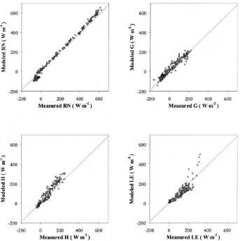
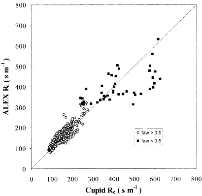
Fig. 2. Comparison of primary energy flux component measurements made during MONSOON ’90 with estimates from the ALEX model.
improves the agreement with both models. Compar-isons between ALEX predictions of canopy and soil temperature and evaporation and measurements are contained in Fig. 3. Here, the component evaporation measurements have been adjusted such that they sum to the closure-corrected system evaporation flux while maintaining the measured soil/canopy partitioning ra-tio. Again, the performance is similar to that of Cupid; both show a tendency to under-predict transpiration, perhaps due to residual problems with the modified Ball et al. (1987) at low humidities.
4.3. Canopy resistance and light-use efficiency
Canopy resistance estimates from ALEX and Cupid simulations, using meteorological inputs from FIFE
’87, are compared in Fig. 4. In Cupid,Rcis computed as a leaf-area-weighted summation ofRs,leaf over all
leaf angle and layer classes in the canopy. The analyt-ical model forRcdeveloped here produces values that agree well with those derived numerically by Cupid. Note that the dry-down that occurred during the 3rd IFC (faw<0.5) effected significant stomatal closure in
both models.
and VPD is low, are also found in the modeled efficiencies.
4.4. Carbon and evapotranspiration fluxes
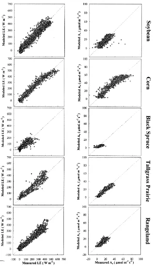
Carbon assimilation and evapotranspiration fluxes simulated with the ALEX model, using inputs listed in Table 2, are compared with hourly eddy covari-ance measurements in Fig. 6; Table 3 provides a
Table 3
Quantitative measures of model performance in estimating hourly carbon and heat fluxesa
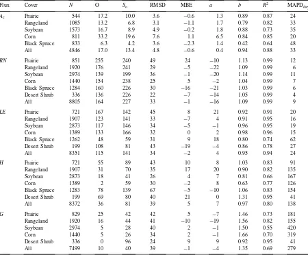
Flux Cover N O So RMSD MBE a b R2 MAPDday
Ac Prairie 544 17.2 10.0 3.6 −0.6 1.3 0.89 0.87 24
Rangeland 1085 13.2 6.8 3.1 −1.1 1.7 0.79 0.82 33
Soybean 1573 16.7 8.9 4.9 −0.2 1.8 0.88 0.73 35
Corn 811 33.2 19.6 7.6 1.1 6.5 0.84 0.85 20
Black Spruce 833 6.3 4.2 3.6 −2.3 1.4 0.42 0.64 48
All 4846 17.0 13.4 4.8 −0.6 0.4 0.94 0.88 33
RN Prairie 851 255 240 49 24 −10 1.13 0.99 12
Rangeland 1920 176 241 29 −5 −22 1.09 0.99 6
Soybean 2974 139 199 36 −1 −20 1.14 0.99 11
Corn 1440 154 238 25 5 −2 1.04 0.99 7
Black Spruce 1284 160 226 30 −16 −21 1.03 0.99 6
Desert Shrub 336 136 226 22 −7 −14 1.05 0.99 4
All 8805 164 227 33 −1 −16 1.09 0.99 9
LE Prairie 721 167 142 45 8 21 0.92 0.91 20
Rangeland 1907 123 141 33 −7 4 0.91 0.95 16
Soybean 2873 117 146 34 −5 −1 0.96 0.95 19
Corn 1389 133 166 32 0 2 0.98 0.96 15
Black Spruce 1262 48 59 31 9 18 0.80 0.74 62
Desert Shrub 199 108 81 43 −19 −4 0.86 0.78 27
All 8351 115 141 34 −2 4 0.95 0.94 24
H Prairie 721 55 89 43 10 8 1.03 0.83 91
Rangeland 1907 31 70 35 17 20 0.90 0.82 135
Soybean 2873 18 41 26 4 7 0.81 0.66 167
Corn 1389 2 59 30 −2 8 0.63 0.77 126
Black Spruce 1283 78 139 67 −5 −10 1.06 0.83 154
Desert Shrub 199 69 80 40 21 0 1.31 0.95 41
All 8372 36 81 39 5 7 0.97 0.80 138
G Prairie 829 25 42 42 5 −7 1.46 0.73 181
Rangeland 1920 16 44 41 −10 −19 1.56 0.82 155
Soybean 2974 5 28 40 2 −1 1.50 0.55 420
Corn 1440 5 26 34 2 −1 1.66 0.70 319
Desert Shrub 336 0 96 24 9 9 0.92 0.95 41
All 7499 10 40 39 −1 −4 1.35 0.69 279
aHere N is the number of observations, O and So are the mean and standard deviations of the observations, RMSD is the root-mean-square-difference between the modeled (P) and observed (O) quantities, MBE is the mean-bias-error,aandbare the intercept and slope of the linear regression ofPonO,R2 is the coefficient of determination, and MAPDdayis the mean-absolute-percent-difference between daytime observations and model predictions. The termsN,b,R2and MAPDdayare unitless;O,So, RMSD, MBE, andahave units ofmmol m−2s−1 forAcand units of Wm−2 forRN,LE,HandG.
statistical description of these compansons. Included here are the root-mean-square-difference (RMSD), and the daytime mean-absolute-percent-difference (MAPDday), defined as the absolute value of the
Fig. 3. Comparison of predicted soil-surface and vegetation evap-oration rates and temperatures with measurements from MON-SOON ’90.
Hourly carbon flux comparisons in Fig. 6 and Table 3 have been restricted to daytime hours (solar irradia-tion > 50mmol m−2s−1), while comparisons of latent
heat fluxes include day and nighttime measurements. As evident in Fig. 6, the analytical canopy resis-tance submodel in ALEX does reasonably well at reproducing measured carbon and water fluxes on an hourly timescale. Its success is particularly notable
Fig. 4. Comparison of canopy resistance values predicted by the ALEX and Cupid models for flux measurements obtained during FIFE ’87.
given the simplicity of the model and the limited number of tunable parameters it requires. The mea-surements displayed here represent a wide range in atmospheric, soil moisture, and phenological con-ditions. The effects of stomatal closure during the dry-down in the 3rd FIFE IFC, for example, are well-reproduced by the soil moisture stress term (faw,
Eq. (16)). During this interval,fawvaried between 0.4
and 0.9. If soil moisture effects are ignored during this IFC, Ac is overestimated by up to 25mmol m−2
s−1, andLEby 250 W m−2.
The MAPDday statistic in Table 3 permits
Fig. 5. A time-course of measurements of effective light-use efficiency and carbon assimilation measurements made in corn over eight consecutive days (lines). Also plotted are simulated values of LUE andAcgenerated by the ALEX model (circles).
carbon flux systems used during FIFE ’89 showed 5–15% variations (Moncrieff et al., 1992).
In comparison, the MAPDdayvalues for hourly
day-time flux estimates from the ALEX model, averaged over the six datasets represented in Table 3, are 9% (RN), 24% (LE), and 33% (Ac). The errors inRNand LEare comparable to observational errors encountered during FIFE. While the model RMSD forAcis signif-icantly larger than the expected error, theR2value of 0.88 is encouraging. Some of the scatter in the canopy assimilation comparisons is introduced by the empiri-cal soil respiration correction to measured system car-bon fluxes. Other important sources of error include inaccurate specification of green leaf area, and the use of a net LUE based on seasonal NPP measurements (see further).
Sensible and soil heating fluxes are less accu-rately determined from a MAPD standpoint. While
the RMSD for all energy flux components is roughly equal on average (35–40 W m−2), the low average magnitudes of HandG lead to high MAPDday
val-ues of 138 and 279%, respectively. The amplitude of the diurnal soil heat flux curve is consistently overestimated by ALEX, with the exception of the MONSOON ’90 database. A calibration in sand of 14 different commercially-available soil heat flux plates conducted by Twine (1998) revealed that the plates consistently under-measured the known flux under both saturated and dry conditions. Translated to thermal conductivities typical of the FIFE site, for example, the expected bias is on the order of 5%. This may explain in part the disagreement be-tween the modeled and measured diurnal soil flux amplitudes. In the ALEX formulation, Hc and Hs
Fig. 7. Comparison of daily-integrated measurements of system latent heating and canopy carbon assimilation made in six different vegetative stands with estimates generated by the ALEX model.
values for G tend to accumulate in H, leaving LE unaffected.
Because we have used LUE values based on sea-sonal dry matter accumulation, we expect Eq. (11) to underestimate daytime hourly carbon fluxes to some degree (see Section 3.3). This effect is particularly evident for black spruce (Fig. 6), which has a high
Table 4
Quantitative measures of model performance in estimating daily-integrated carbon and heat fluxesa
Flux N O So RMSD MBE a b R2 MAPD
Ac 102 37.9 22.4 6.7 −0.1 0.0 1.00 0.92 18 RN 166 13.3 3.8 0.8 −0.3 −0.4 1.01 0.96 6 LE 128 9.9 3.1 1.3 −0.4 0.4 0.92 0.85 12 H 135 2.9 2.8 1.6 0.6 1.1 0.81 0.71 197 G 142 0.7 0.9 0.8 −0.1 0.0 0.80 0.46 161
aN, O, So, RMSD, MBE, a, b and R2 are defined as in Table 1. MAPD is the mean-absolute-percent-difference between observed and modeled daily-integrated fluxes. The termsN,b,R2 and MAPD are unitless;O,So, RMSD, MBE, andahave units of gC per day forAcand units of MJ per day forRN,LE,HandG.
18% (Ac). We note that net carbon fluxes over black spruce are still underestimated, even in a daily aver-age. For reasonable daily estimates of carbon uptake, the net LUE for spruce must be adjusted to compen-sate for seasonal variations in the respiration to assim-ilation ratio.
5. Conclusions
A simple analytical model for predicting carbon assimilation fluxes and canopy transpiration based on stand-level measurements of canopy LUE has been de-veloped and tested in comparison with measurements made over canopies of a variety of C3 and C4 plant
species. Comparisons between modeled and mea-sured evapotranspiration (LE) and carbon assimilation (Ac) fluxes yield mean-absolute-percent-differences
of 24% (LE) and 33% (Ac) for hourly daytime fluxes,
and 12% (LE) and 18% (Ac) for daily-integrated
fluxes. The analytical model also reasonably captures observed phenomena such as moisture stress effects on stomatal conductance and modulation of canopy LUE due to diurnal variations in insolation composi-tion and VPD.
With these measurement datasets, we found that the simple semi-empirical model described here per-formed as well and often better than the more detailed, process-based Cupid model. This finding illustrates an interesting point made by Jarvis (1993), who notes that ‘bottom-up models’, constructed from detailed mechanistic representations of leaf-level processes and scaled to the canopy level, are often more susceptible to errors in inputs and scaling assumptions than are
‘top-down’ models, which are constrained ‘to the realm of observation’ by some relationship developed at the stand level. In the simple model, assimilation (and therefore canopy resistance) is semi-constrained (but not rigidly fixed) by a quantity that has been found to be conservative in nature: the canopy LUE. Even if small errors occur on an hourly timestep, the daily or seasonal integral of carbon uptake will gener-ally be properly constrained under this approach, and these are in many applications the flux timescales of interest.
Jarvis (1993) warns, however, that top-down mod-els such as this have usefulness only within the range of conditions under which the embedded empiricisms were developed. We have no assurance, for example, that this model as it is given here will perform well in predicting regional fluxes under conditions of el-evated CO2. For such studies, a synthesis between
top-down and bottom-up modeling may be optimal. A process-based model such as Cupid can be used to modify slowly-evolving empirical relationships (such as theβ versus Ci relationship in Eq. (10))
embed-ded in the analytical model, which can then be em-ployed more efficiently at finer spatial and temporal resolution.
Acknowledgements
Appendix A. The ALEX model
ALEX, in its most basic form, is a two-source (soil and vegetation) model of heat, water and carbon ex-change between a vegetated surface and the atmo-sphere. The net energy balance at the earth’s surface can be represented by
RN=H+LE+G (A.1)
whereRNis the net radiation above the surface, and H,LE, andGare the fluxes of sensible, latent, and soil conduction heating, respectively. The set of equations defining energy fluxes (W m−2) in the ALEX model
(see Fig. 1) is as follows:
Net Radiation:
RN=RNc+RNs (A.2)
RNc=Hc+LEc (A.3)
RNs=Hs+LEs+G (A.4)
Sensible Heat:
H =Hc+Hs (A.5)
H =ρcp
Tac−Ta Ra
(A.6)
Hs=ρcp
Ts−Tac Rs
(A.7)
Hc=ρcp
Tc−Tac
Rx (A.8)
Latent Heat:
LE=LEc+LEs (A.9)
LE=ρcpeac−ea
γp Ra
(A.10)
LEs =ρcpes−eac
γp Rs
(A.11)
LEc=LEce+LEct (A.12)
LEce =
ρcpe∗(Tc)−ea γp Rx/fwet
(A.13)
LEct =f[Tc, eac] (Light-use efficiency submodel)
(A.14)
Soil Heat:
G=f[T (z), θ (z)] (Soil transport submodel) (A.15)
whereTis temperature (K),eis vapor pressure (kPa), Ris the transport resistance (s m−1),ρ is the density of air (kg m−3),cpis the heat capacity of air at
con-stant pressure (J kg−1K−1) andγpis the
psychomet-ric constant (kPa K−1).
The subscripts ‘a’, ‘ac’, and ‘x’ signify properties of the air above and within the canopy, and within the leaf boundary layer, respectively, while ‘s’ and ‘c’ refer to fluxes and states associated with the soil and canopy components of the system. The resistance terms (R) are defined in the main text (Section 3.1; note that in Section 3, resistance is expressed in units of m2smmol−1).
The soil and canopy energy budgets are fueled by the net radiation apportioned to each component (RNs andRNc, respectively). In ALEX, we have adopted a simple, analytical method for partitioning net radiation that depends on leaf and soil optical properties and on the canopy leaf area index; this strategy is outlined in Appendix B.
Canopy transpiration (LEct) and soil heat
conduc-tion (G) flux estimates are generated by submodels within ALEX, as indicated by the functional expres-sions in Eqs. (A.14) and (A.15). The transpiration submodel is described in Section 3.1 in the main text. The flux of heat conducted into the soil surface is computed by a multi-layer numerical soil model that serves as the lower boundary to ALEX, described briefly further (Section A.l). This model also provides an estimate of the vapor pressure at the soil surface (es), used in predicting the soil evaporation rate (Eq. (A.11)). The canopy evaporation flux (LEce) arises from the fraction of total leaf area (F) that is covered by liquid water (fwet), as discussed in Section A.2.
A.1. Soil transport submodel
equations using a Newton–Raphson finite-difference solution technique. The temperature and water content at the soil surface form the interface condition between transport in the soil and exchanges in the vegetative canopy.
A.1.1. Heat
The soil temperature profile (including the surface temperature Ts) and the conduction flux of heat
through the soil profile (including the surface heat flux, G) are obtained as the solution to the time-dependent differential equation for heat flow:
ρscs surface (m); ρscs is the volumetric soil heat
capac-ity (J m−3K−1), λs is the soil thermal conductivity
(J m−1s−1K−1),QH is the heat source term given by (RNs−LEs)/1z(W m−3) at the soil surface and1z
is the thickness of the surface soil layer (m). The soil surface heat flux is obtained by integrating Eq. (A.16) over the surface layer:
Because thermal conductivity is a non-linear func-tion of soil water content, the system of layer tem-perature equations (A.16) must be solved in iteration with the soil water profile.
A.1.2. Water
The time rate of change in soil water content with depth is given by Richard’s Equation:
∂θ
where θ is the volumetric water content (m3m−3), Kw is the soil hydraulic conductivity (kg s m−3); ψ is the soil water potential (J kg−1), g is the grav-ity (m s−2), Kwgis the drainage due to gravitational
forces (kg m−2s−1) and U is the volumetric water sink (kg m−3s−1). At the soil surface,Uaccounts for
the difference between soil evaporation and infiltra-tion rates. Below the surface, it represents the water extracted from a given soil layer by plant roots.
Plants will extract the most water from those soil layers that contain the greatest density of roots (Camp-bell, 1985). Roots tend to have an exponential distri-bution with depth in the soil, so the fraction of active roots between depthzand depthz+1zcan be approx-imated with
Froot(z)=e
−τ z−e−τ (z+1z)
1−e−τ dr (A.19)
wheredr is the depth of rooting (m) andτ is the em-pirical distribution coefficient (Norman and Campbell, 1983).
This distribution scheme places most of the roots in the upper layers of the soil, as has been observed in many studies. As written,Froot(z) is normalized to
sum to unity over the rooting depth (dr). If any layer
of thickness ∆z is depleted of available water, then dr in Eq. (A.19) is replaced by dr−∆z, andFroot (z)
for that layer becomes zero. The root uptake function used in ALEX is
whereλkis the latent heat of vaporization (J kg−1) and LEct′ is the transpiration rate reduced by soil water
limitations (W m−2; Eq. (17) in the main text). Under heavy rainfall, the cumulative precipitation transmitted to the soil surface during a given timestep may exceed the surface infiltration capacity. In such cases, the excess water can either be temporarily ponded and saved for infiltration during subsequent tiinesteps, or it can be extracted from the modeling site in the form of runoff. The fate of excess water is likely to be determined by the local topography of the site: whether it is on a slope or in a basin. In ALEX, we define a soil surface storage capacity: the maxi-mum depth of water,hmax (mm), that can be stored on the surface before runoff occurs. If the site is in a basin where ponding is allowed, surface storage is effectively unlimited. If not, the soil water potential at the soil surface is constrained to be less than or equal to some small positive value corresponding to the headhmax. The surface source term in Eq. (A.18)
A.2. Canopy evaporation/dew deposition
During light precipitation events over a dense canopy, there can be significant potential for inter-ception and re-evaporation of rain or irrigation waters over relatively short time scales. Following Sellers et al. (1996), the maximum canopy interception store (Wimax; mm) is presumed to be a linear function of
the leaf area index (F):
Wi max=2×Wi max×F, (A.21)
whereWimax is the maximum potential reservoir (in
mm) per unit single-sided leaf area, and we assume that both sides of each leaf will be wetted equally. Inci-dent precipitation (Wo) is partitioned between canopy
interception and soil application based on the vegeta-tion cover fracvegeta-tion (fc) until this interception reservoir is filled:
Wi=min(fc×Wo, Wi max); (A.22)
any additional precipitation is transmitted to the soil surface and attributed toU(Eq. (A.18)). For precipi-tation falling vertically, the relevant cover fraction is an exponential function of leaf area index:
fc=1−exp(−0.5F ) (A.23)
where we have assumed a random, spherical leaf angle distribution.
Intercepted water typically will not coat the leaf uniformly; beads tend to form, leaving parts of the leaf free from standing water and stomata unblocked to transpiration and assimilation fluxes. In ALEX, the fraction of leaf area covered with water (fwet) grows
linearly with intercepted precipitation to some maxi-mum allowed value (fwet max) attained when the
inter-ception reservoir is filled (Wi=Wi max) the remainder of the canopy is presumed to be dry:
fwet = Wi Wi max
fwet max, (A.24)
fdry=1−fwet. (A.25)
The boundary layer resistance to evaporation from this leaf-surface water pool must take this wetted leaf area fraction into account:
LEce=
ρcp[e∗(Tc)−eac] λ Rx/fwet
. (A.26)
When conditions in the canopy are conducive to dew deposition (e*(Tc)<eac), the total leaf area
par-ticipates and the factor fwet is omitted from Eq.
(A.26).
Appendix B. Approximations for net radiation and absorbed PAR
Net radiation and absorbed PAR are modeled in ALEX using an analytical formalism describing light interception by canopies developed by Goudriaan (1977) and outlined by Monteith and Unsworth (1990) and by Campbell and Norman (1998). Assuming that the leaf reflectance and transmittance factors are equal, simple approximations for canopy reflectance and transmittance can be constructed involving only leaf absorptivity, soil reflectance, canopy leaf area in-dex (LAI) and leaf angle distribution (LAD). Goudri-aan (1977) showed that these approximations work well over a range of leaf and canopy properties, and for solar zenith angles less than the mean leaf inclina-tion angle (60◦in the case of a spherical LAD). They include the effects of reflection at the soil surface and re-reflection by leaves, which can be important in sparse canopies, serving to enhance the downwelling radiation field.
Given measurements or estimates of LAI, LAD, leaf absorptivity in the visible, near infrared (NIR) and thermal wavebands, and soil reflectance in the visible and NIR, canopy transmittance factorsτbv,τdv,τbn, τdn, and τdl, and reflectance factors ρbv, ρbn, ρdn,
andρdlcan be computed using these approximations.
Here, subscripts ‘v’, ‘n’, and ‘l’ signify the visible, NIR and thermal wavebands, and subscripts ‘b’ and ‘d’ indicate response to direct beam and diffuse radia-tion components, respectively. Vegetaradia-tion clumping in canopies can be accommodated by modifying the LAI used in the calculation of extinction coefficients by a ‘clumping factor’ (Chen and Cihlar, 1995; Campbell and Norman, 1998).
Weiss and Norman (1985) summarize a methodol-ogy for partitioning measurements of solar irradiance (S) into visible and NIR waveband components (Sv
andSn), and further into diffuse and direct beam
com-ponents (Sdv, Sdn, Sbv, and Sbn). Using the resulting
fv=
a radiation-weighted surface albedo can be obtained:
αsfc=fv(fdv×ρdv+fbv×ρbv)
+fn(fdn×ρdn+fbn×ρbn) (B.2)
Given these canopy reflectance and transmittance coefficients and estimates of the soil reflectivity in the visible, NIR and thermal wavebands (ρsv, ρsn, and ρsl, respectively), the net radiation above the canopy (RN) and above the soil surface (RNs), and the diver-gence of net radiation within the canopy (RNc) can be
approximated with
The longwave components of RNandRNs are
func-tions of the thermal radiation emitted by the sky (Lsky = εskyσ Ta4, whereσ is the Stefan-Boltzmann
coefficient andεskyis the sky emissivity), the canopy
(Lc = εcσ Tc4; εc is the canopy emissivity) and the
soil (Ls =εsσ Ts4;εs is the soil emissivity). Here we
have retained only those components that are first or lower order in thermal reflectivity; however, because the coefficient of diffuse thermal radiation transmis-sion through the canopy will approach unity for sparse vegetation, the second order component inτdlis also
retained. Following Monteith and Unsworth (1990), atmospheric emissivity is approximated as a weighted average of clear and cloudy values, weighted by the fraction of sky cloud cover. We use the empirical formula of Brutsaert (1984) for estimating clear sky emissivity, and assume a cloud emissivity of 1. The soil emissivity is given byεs=1−ρsl, and the canopy
emissivity byεc=1−ρdl−τdl. The shortwave
com-ponents of net radiation depend on insolation values
above the canopy (S) and above the soil surface, the re-flectivity of the soil-canopy system (αsfc) and the soil
surface in the visible and NIR bands (ρs,vandρs,n).
The PAR radiation absorbed by green leaves in the vegetation canopy can be approximated with
PAR=fvSA
Anderson, M.C., Norman, J.M., Diak, G.R., Kustas, W.P., Mecikalski, J.R., 1997. A two-source time-integrated model for estimating surface fluxes using thermal infrared remote sensing. Remote Sensing Environ. 60, 195–216.
Aphalo, P.J., Jarvis, P.G., 1991. Do stomata respond to relative humidity? Plant, Cell Environ. 14, 127–132.
Avissar, R., Pielke, R.A., 1991. The impact of plant stomatal control on mesoscale atmospheric circulations. Agric. For. Meteorol. 54, 353–372.
Baldocchi, D., 1994. An analytical solution for coupled leaf photosynthesis and stomatal conductance models. Tree Physiol. 14, 1069–1079.
Baldocchi, D.D., Meyers, T.P., 1998. On using ecophysiological, micrometeorological and biogeochemical theory to evaluate carbon dioxide, water vapor and trace gas fluxes over vegetation: a perspective. Agric. For. Meteorol. 90, 1–26.
Ball, J.T., 1988. An analysis of stomatal conductance. Ph.D. Thesis, Stanford University.
Ball, J.T., Woodrow, I.E., Berry, J.A., 1987. A model predicting stomatal conductance and its contribution to the control of photosynthesis under different environmental conditions. In: Biggins, J. (Ed.), Progress in Photosynthesis Research. Nijhoff, Dodrecht, pp. 221–225.
Brutsaert, W., 1984. Evaporation into the Atmosphere: Theory, History and Applications. D. Reidel, Boston.
Campbell, G.S., 1985. Soil physics with BASIC — Transport Models for Soil–Plant Systems. Elsevier, New York. Campbell, G.S., Norman, J.M., 1998. An Introduction to
Environmental Biophysics. Springer, New York.
Chen, J.M., Cihlar, J., 1995. Quantifying the effect of canopy architecture on optical measurements of leaf area index using two gap size methods. IEEE Trans. Geosci. Remote Sensing 33, 777–787.
Collatz, G.J., Ball, J.T., Grivet, C., Berry, J.A., 1991. Physiological and environmental regulation of stomatal conductance, photosynthesis and transpiration: a model that includes a laminar boundary layer. Agric. For. Meteorol. 54, 107–136. Collatz, G.J., Ribas-Carbo, J., Berry, J.A., 1992. Coupled