ON THE QUALITY AND EFFICIENCY OF APPROXIMATE SOLUTIONS TO BUNDLE
ADJUSTMENT WITH EPIPOLAR AND TRIFOCAL CONSTRAINTS
Johannes Schneider, Cyrill Stachniss and Wolfgang F¨orstner
Institute of Geodesy and Geoinformation, University of Bonn (johannes.schneider, cyrill.stachniss, wolfgang.foerstner)@igg.uni-bonn.de
KEY WORDS:Bundle Adjustment, Trifocal Constraint, Approximate Solution, Quality Evaluation
ABSTRACT:
Bundle adjustment is a central part of most visual SLAM and Structure from Motion systems and thus a relevant component of UAVs equipped with cameras. This paper makes two contributions to bundle adjustment. First, we present a novel approach which exploits trifocal constraints, i.e., constraints resulting from corresponding points observed in three camera images, which allows to estimate the camera pose parameters without 3D point estimation. Second, we analyze the quality loss compared to the optimal bundle adjustment solution when applying different types of approximations to the constrained optimization problem to increase efficiency. We implemented and thoroughly evaluated our approach using a UAV performing mapping tasks in outdoor environments. Our results indicate that the complexity of the constraint bundle adjustment can be decreased without loosing too much accuracy.
1. INTRODUCTION
Precise models of the environment are needed for several robotic applications and are central to several UAV-based services. Most SLAM and visual mapping systems use a form of bundle adjust-ment (BA) for simultaneously refining camera pose parameters and 3D point coordinates. Thus, effectively solving the BA or the underlying error minimization problem is essential for many ap-proaches such as structure from motion (Agarwal et al., 2011) and online SLAM or visual odometry. BA has favorable properties: it is statistically optimal in case all statistical properties are mod-eled and considered correctly, it is efficient in case sparse matrix operations are used, and can be parallelized. A broad review is given by Triggs et al. (2000).
Steffen et al. (2010) have shown that rigorous BA can be formu-lated based only on epipolar and trifocal constraints. The epipolar constraint is a relation between two camera views, that enforces an image point to be on the epipolar line described by an corre-sponding image point in another image and the essential or funda-mental matrix between the views (Hartley and Zisserman, 2004). A trifocal constraint between image points is necessary if the cor-responding scene point lies on the trifocal plane, which practi-cally always is true for neighbored images in an image sequence, where projection centers are collinear or nearly collinear. Epipo-lar and trifocal constraints lead to implicit functions that enforce the intersection of bundle of rays in 3D space without explicitly representing 3D point coordinates. This reduces the number of unknown parameters of the underlying optimization problem to the camera pose parameters. The obtained normal equations are equivalent to the normal equation system of classical BA when applying the Schur Complement to eliminate the unknown 3D point coordinates. Its solution is therefore in statistical terms as optimal as classical BA.
BA based only on epipolar and trifocal constraints has several advantages over classical BA:
• it allows to integrate image points, whose projections rays have small parallactic angles, which in classical bundle ad-justments would lead to 3D points lying numerically at in-finity. Including such observations increases the generality
of BA and improves the estimated rotations of the camera pose parameters (Schneider et al., 2012);
• it leads directly to the normal equation system reduced to the camera pose parameters. Classical BA needs to apply the Schur Complement to eliminate the 3D points;
• it does not require an initial guess for the locations of the 3D points, which is required for classical BA;
• it allows to arrive at approximate solutions, e.g., by neglect correlations between multi-view constraints and the relin-earization of observations, which significantly increases the efficiency without a substantial loss in accuracy.
Nevertheless, the trifocal BA formulation without simplifying ap-proximations leads to higher computational complexity than clas-sical BA. Because of the implicit epipolar and trifocal constraints one needs to employ the Gauss–Helmert Model for optimization, which requires the costly determination of corrections for all ob-servations, which is not needed in the Gauss–Markov Model em-ployed for classical BA. To substantially reduce the computa-tional complexity Indelman et al. (2012) propose to neglect (1) correlations between the constraints and (2) corrections to the observations during optimization and (3) fix the weights for the individual constraints after the first iteration.
In this paper we investigate (1) the gain in efficiency and (2) the loose of quality of several assumptions, which lead to an approx-imate solution of BA which substantially reduces computational complexity. Additionally we propose a new formulation for tri-focal constraints which can be employed in BA without struc-ture estimation. Contrary to formulations of trifocal constraints in previous work it does not degenerate in specific situations.
2. RELATED WORK
which exploits the sparse secondary structure of sparse camera to camera relations, which increases computational and mem-ory efficiency. More recently, the popular software package g2o (K¨ummerle et al., 2011) shows a comparable efficiency as sSBA but uses a more generic formulation of the optimization problem using factor graphs.
BA without structure estimation has been proposed by Rodr´ıguez et al. (2011), but their approach relies only on epipolar con-straints, which are not able to transfer a consistent scale between cameras having parallel epipolar planes which occur on straight camera trajectories. Thus Steffen et al. (2010) propose to use epipolar and trifocal constraints in BA without structure estima-tion. But their trifocal constraints can not be computed in a closed form expression which is why a stable condition needs to be sam-pled, where the number of samples is not fixed. Indelman et al. (2012) propose simplifying approximations to the optimiza-tion problem by rewriting the implicit trifocal and epipolar con-straints into explicit expressions. This way the authors obtained a pose graph formulation, which can be optimized with the com-putational efficient incremental smoothing and mapping (iSAM) algorithm by Kaess et al. (2012). But their approach can not han-dle all possible camera configurations.
3. CLASSICAL BUNDLE ADJUSTMENT
The general objective of BA is to optimally estimate camera ro-tationsRbt, camera positionsZbtand 3D point coordinatesXbi si-multaneously. In the following, we assume that each observed 2D image pointxitin viewtis associated to a certain 3D pointiand that the intrinsic camera calibration is given by calibration ma-trixKt. Given an initial guess, i.e., knowing approximate quan-titiesRbat,Zbat andXbai, the reprojection with projection matrix
yields the homogeneous image point
xait=PatX a
i. (1)
With the three rows P1,t, P2,t and P3,t of Pt we obtain the reprojected image point in Euclidean coordinates xait = h
P1,tXbai/P3,tXbai,P2,tXbai/P3,tXbai iT
and the reprojection error
vit=xait−xitin the image plane. Assuming the image points to be corrupted with mutually uncorrelated Gaussian noiseΣxitxit, maximum likelihood estimates are obtained by iteratively im-proving the unknown parameters by minimizing the squared Ma-halanobis distancePitvT
itΣ− 1
xitxitvitusing the Gauss–Markov model, see (F¨orstner and Wrobel, 2016, Sect. 4.4).
WithTcamera poses andIobserved 3D points, the total number of unknown parameters to be optimized counts6T+ 3I. If one is only interested in estimating the camera poses, the normal equa-tion system can be reduced to the6Tpose parameters by applying the Schur complement. However, as BA needs to be solved iter-atively due to its non-linearity one is forced to compute the 3D point in each iteration, even if they are not of interest. In contrast to that, we can directly obtain the reduced normal equation sys-tem without applying the Schur complement or determining 3D points by employing epipolar and trifocal constraints, which are introduced in the next section.
4. EPIPOLAR AND TRIFOCAL CONSTRAINTS
The classical solution to BA seeks to minimize the reprojection error of corresponding points. Alternatively, we can formulate
X
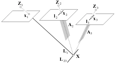
Figure 1. Trifocal constraint. We choose two linesl2andl3 through the image pointsx2andx3of the second and third camera. The corresponding projection planesA2andA3raise the intersection lineL23. The constraint requires that projection
lineL1and intersection lineL23intersect in one single point.
an error minimization problem that exploits constraints from the epipolar geometry of image pairs as well as constraints that re-sult from observing the same point from three different camera images, so-called trifocal constraints. This formulation has the advantage, that only the camera extrinsics are unknown parame-ters and we do not need to estimate the 3D point parameparame-ters in the optimization. After describing how to formulate such constraints in this section, we explain in Sec. 5 how to consider them in BA.
Given three corresponding image points (x1,x2,x3) in three viewst = 1,2,3, we need to formulate three independent con-straints (g1, g2, g3) for each correspondence related to a 3D point. Two-view epipolar constraints do not allow to transfer a consis-tent scale given straight trajectories with collinear projection cen-ters (Rodr´ıguez et al., 2011), which usually appear in image se-quences. We always use one trifocal and two epipolar constraints, which are simpler and one trifocal constraint is sufficient.
Thefirst two constraintsare epipolar constraints and enforce the camera rays to be on their epipolar lines w.r.t. the first camera
g1=xT1RT1S(Z2−Z1)R2x2 (2) g2=xT1RT1S(Z3−Z1)R3x3, (3)
whereS(·)is the skew symmetric matrix of the input vector. Note
that we assume here, that the the camera calibration is given, such that we can convert an image point x into a ray direc-tionx, e.g.in case of a pinhole camera with calibration matrixK
byx=K−1
xT,1T
.
Thethird constraintenforces the intersection of all ray directions in a single point, which we formulate in the following way. Con-sider two planesA2 andA3 that go along the ray directionx2 andx3and are projected as 2D linesl2andl3such that we have
A2 =PT2l2 andA3 =PT3l3, see Figure 1. The intersection of both planes in 3D yields the 3D line
L23= I I(A2)A3 with I I(A) = along the ray directionx1
L1=
coor-dinates this leads to the constraint
g3=LT1DL23 with D= 0 I
3
I3 0
. (6)
whereDis the dualizing matrix.
We need to guarantee thatL1intersectsL23in one single point. In order to achieve a numerically stable constraint we choose the two linesl2 andl3 and specify their directionv2 andv3 to be perpendicular to the epipolar lines in the second and third image, such that we have
l2=S(v2)x2 with v2=S(RT2(Z2−Z1))x2, (7)
l3=S(v3)x3 with v3=S(RT3(Z3−Z1))x3. (8)
When using the constraintg3in an estimation procedure, the vec-torsv2andv3can be treated as fixed entries.
These constraints work for all points if they are not close to an epipole, which would also not work in a classical BA. Then at least two projection planes are nearly parallel and the intersect-ing line is numerically unstable or, in case of observational noise, inaccurate. This especially holds for forward motion, for which image points close to the focus of expansion, i.e. the epipole, can-not be handled.
If none of the image points are close to the epipoles, then, follow-ing Figure 1, the two projection planesA2andA3of the second image intersect the projection lineL1 of the first image in well defined points and are not parallel, thus have a well defined in-tersection lineL23, which therefore needs to pass the projection lineL1. Hence, the triplet constraint never has a singularity and fixes the image pointsx2 andx3 perpendicular to the epipolar lines w.r.t. the first image used in Eq. (2) and (3).
Indelman (2012) uses the trifocal constraint
z3= (S(R2x2)R1x1)TS(R3x3)(Z3−Z2) (9)
−(S(R1x2)(Z2−Z1))TS(R3x3)R2x2,
but this formulation degenerates in case the epipolar plane nor-malsn12andn23of first and second camera and second and third camera are perpendicular. The constraint projects normal direc-tionn12given with different lengths in Eq. (9) byS(R2x2)R1x1 andS(R1x2)(Z2−Z1)on normal directionn23given with dif-ferent lengths byS(R3x3)(Z3−Z2)and S(R3x3)R2x2. In case of perpendicular normal directions, the constraint would be fulfilled under multiple solutions.
So far we have only considered three-view correspondences. In case of correspondences in less than three view we can only apply the epipolar constraint (2). In case ofNi>3correspondences, we need to avoid to use the same constraints twice, and use only independent constraints between the different views. Each cor-responding image observation contributes with two constraints, therefore the total number of constraints between corresponding views counts(2Ni−3). Each correspondence needs to be in-volved in at least one epipolar and one trifocal constraint. In-delman et al. incorporate an new image of an image sequence by formulating epipolar constraints between the last two recent im-ages and trifocal constraints between the last three recent imim-ages.
As in a classical BA the estimation of the poses of calibrated cam-eras is only possible up to a similarity transformation. To over-come the 7 DOF ambiguity of the overall translation, rotation and
scale, we define either the gauge by imposing seven centroid con-straints on the approximate values of the projection centers. This results in a free BA, where the trace of the covariance matrix of estimated camera poses is minimal. Or we estimate the camera poses relative to one camera, which fixes six DOF. To define the overall scale, we constrain two cameras to have a certain distance to each other, see (F¨orstner and Wrobel, 2016, Chapt. 4.5).
5. TRIFOCAL BUNDLE ADJUSTMENT
We sketch the maximum likelihood estimation with implicit func-tions, also called estimation with the Gauss–Helmert model, see (F¨orstner and Wrobel, 2016, Chapt. 4.8) and relate it to the clas-sical regression model, also called Gauss–Markov model. This is the basis of four variants for simplifications. These lead to ap-proximations which are then compared with the statistically opti-mal ones w.r.t. accuracy and speed of convergence.
5.1 The Estimation Model
5.1.1 Gauss–Helmert Model The Gauss–Helmert model starts fromGconstraints,g = [gg], among theN observations
l = [ln], which are assumed to be a sample of a multivariate Gaussian distributionN(IE(l), σ2
0Σ a
ll), andUunknown parame-tersx= [xu]:
g(IE(l),x) =0 and ID(l) =σ02Σ a
ll. (10)
We assume the covariance matrix of the observations is approxi-matelyΣall, hence we assumeσ0= 1; we will be able to estimate this factor later. Given observationsl= [ln]there are no param-etersxfor whichg(l,x) = 0holds. Therefore the goal is to find correctionsbvof the observations and best estimatesxbsuch that the constraints
g(bl,xb) =g(l+bv,bx) =0 (11)
between the fitted observationsbl=l+vband the estimated pa-rametersxbhold and the weighted sum of the squared residuals
Ω(bl,bx) =vbTΣ−1
ll bv (12)
is minimum.
5.1.2 Solution in the Gauss–Helmert model The solution is iterative. Starting from approximate valuesblaandxbafor the fit-ted observationsbland the estimated parametersbxwe determine corrections∆clandd∆xto iteratively update the fitted observa-tions and the unknown parameters
bl=bla+∆cl=l+vb, xb=bxa+∆dx. (13)
Each iteration solves for the corrections∆cland∆dxwith the lin-earized substitute constraints
g(bl,bx) =g(l,xba) +A∆dx+BT
b
v = 0 (14)
Observe, due to
g:=g(l,x)≈g(IE(l),x) +BTv (15)
we introduce the covariance matrix of the constraints
Σgg=BTΣllB=W− 1
gg (16)
We can determine the corrections in two steps. First, the correc-tionsd∆xare determined from the linear equation system
ATWggAd∆x=ATWggcg with cg=−g(l,xba). (17)
Second, we determine the corrections∆clfrom
c
∆l=ΣllBWgg(cg−Ad∆x)−(bl a
−l), (18)
From Eq. (12) we can determine the estimated variance factor
b σ2
0 = Ω(xb,bl)
R with R=G+H−U (19)
and the weighted sum of the residuals Eq. (12) evaluated at the estimated values
Ω(xb,bl) =bvTWllvb=bcT
gWggbcg. (20)
5.1.3 On the Structure of the Weight MatrixWgg If each constraintgjdepends on one observational grouplj, whose ob-servations are not part of another constraintgj′, the covariance matrixΣgg is diagonal. The same holds, if the constraints can be partitioned into groupsgiwhich only depend on one observa-tional groupli; then the covariance matrixΣggis block diagonal. If the corresponding Jacobians for each group areAT
i andBTi, the matrixNof the normal equation system can be expressed as a
sum over all constraints:
N=ATW
and accordinglyATW
ggcg=PiAi(BTiΣliliBi) −1
cgi.
If a group of constraintsgishares observations, as in our case, the covariance matrixΣgigi=B
T
iΣliliBiwill not be diagonal or
block diagonal any more. Then their inverse, i.e. weight matrix, will be full in general.
For example, in BA, allNi observations referring to the same scene point
X
iwill have a sparse but not diagonal covariance ma-trixΣgigi, hence a full weight matrix of sizeGi×Gi. Let usconsider three epipolar constraintsg = 1,3,5and two trifocal constraintsg = 2,4between the image points of four consecu-tive images,
x
it,t= 1,2,3,4. Then the structure ofBTi for this group of cameras will be as followsBTi =
and the covariance matrix will be
Σgigi = full inverse. Hence, matrixNreads as
N = ATWggA = X
The effort of inverting the generally sparse matrix Σgigi can
be significantly reduced, if the matrix productFi = Wg igiAi
is determined by solving the (generally sparse) equation system
ΣgigiFi=AiforFi.
5.1.4 Solution in the Gauss–Markov Model The solution for the estimated parameters can also be obtained from a Gauss– Markov model when substituting
vg =−BTv (25)
into Eq. (14). Using Eq. (15) andcg from Eq. (17) we immedi-ately obtain the linearized Gauss–Markov model
cg+vg =Ad∆x and ID(vg) =Σgg. (26)
which leads to the same estimates as in Eq. (17).
The iterative solution of this model, however, has to take the lin-earization point for the JacobiansAandBinto account, which
are the fitted observationsbland the the estimated parametersxb. Hence, the result of estimation in the Gauss–Markov model only is the same, if we in each iteration step determine∆clvia Eq. (18) to obtain the fitted original observationsblvia Eq. (13). This is possible, but requires access to the JacobianB. Then there is no
difference between the Gauss–Markov and the Gauss–Helmert model. In addition, we need the inverse of the covariance matrix
Σgg, which in general will not be a diagonal block matrix with small blocks referring to groups of two or three constraints.
These are reasons to investigate approximate solutions, which can be expected to be computationally more efficient.
5.2 Approximations of the Optimal Model
We address four cases of simplifications of the original estimation model. All are approximations of the original model and lead to suboptimal results.
CASEA:Approximated Jacobians
The JacobiansAandBare approximated, bylinearizing at the original observationsl, instead of at the fitted observationsbl. The approximation will increase if the standard deviations of the ob-servations increases, or if there are outliers in the obob-servations. The suboptimality of this approximation has already been dis-cussed in (Stark and Mikhail, 1973).
CASEB:Approximated Weights of the Constraints
The matrixWggis approximated byneglecting the correlations between the constraints. Hence we use the inverse of the diago-nalized covariance matrix,
with the rowsbgofB. This significantly reduces the effort for de-terminingWgg. For CASEB we assume the JacobiansAandB
are taken at the estimated parameters and the estimated observa-tions. This can only be realized within the Gauss–Helmert model, since otherwise the estimated observationsblare not available.
CASE C: Approximated Jacobians and Weights for the Con-straints
CASED:Approximated Weight MatrixWggof the First Iteration
We approximate the weight matrixWggby that obtained in the
first iteration. This reduces the computational burden in the fur-ther iterations.
The weight matrixWggthendepends on the approximate values for the observations and the parameters. Since the approximate values for the parameters usually deviate more from the estimated parameters, than the observations deviate from their fitted values, the degree of approximating the weight matrix by the one of the first iteration mainly depends on the quality of the approximate values for the parameters.
This type of approximation may refer to the full weight matrix or to its diagonal version, as in CASEC. Here, we assume the constraints are treated as uncorrelated. Then we arrive at the same iteration scheme as Indelman et al. (2012).
We will investigate the effect of these four approximations onto the result as a function of the noise level, namely the assumed varianceσ2
0lof the observations, and the varianceσ 2
0xof the ap-proximate valuesxa. In order to be able to make the two standard deviations comparable, we assume they describe relative uncer-tainties with unit 1, for angles units radians. The standard devia-tionσ0lis the directional uncertaintyσl/c, whereσlis the stan-dard deviation of the image coordinates andcthe focal length.
5.3 Generating Approximate Values with a Specified Rela-tive Precision
We perform tests with simulated data by taking the final estimates of real datasets as true values and artificially generate noisy obser-vations and noisy approximate values. In this section we describe how to generate approximate values for the rotation matricesRt
and the positionsZtof the projection centers.
The relative precision of directions or angles is easily specified by their standard deviation measured in radians. Hence if we pre-specify therelative precisionof the approximate values withσ0x, e.g. σ0x = 0.01 = 1 %, we just need to deteriorate the rota-tion axes and rotarota-tion angles by zero-mean noise with standard deviationσα=σ0x.
The relative precision of the coordinates of a set of camera po-sitions, say Zt, is less clear. We propose to use the standard deviation of the direction vectorsDtt′= (Zt−Zt′)/dtt′, with the distancedtt′=|Zt−Zt′|between two neighbouring points
Z
tandZ
t′; here we assume isotropic uncertainty. Furthermore we take relative standard deviation of the distancedtt′ between neighbouring points, i.e. σrtt′ :=σdtt′/dtt′ as measure.There is no obvious way to generate a set of points such that the average relative standard deviation of a given point set fulfills this measure. The following approximation appears sufficient for the experiments. We assume the true values of the camera positions are given byZet. We distort them by taking them as approximate values. Then we generate disturbing observations, namely the coordinate differencesDtt′with a covariance matrix ofID(Dtt′) = σr dtt′I3, withσr = σ0x. We only use pairs (tt′) ∈
T
from a Delaunay triangulation. Since coordinatedif-ferences alone do not allow to estimate the coordinates, we fix the gauge by requiring the sum of all estimated coordinates to
be zero. Therefore we have the following linear Gauss–Markov model with constraints
Dtt′=Zbt′−Zbt, ID(Dtt′) =σ
2 rd
2
tt′ I3, (tt′)∈
T
, (28)0=X
t b
Zt. (29)
MinimizingPtt′|Dtt′|
2
under the constraint leads to estimates b
Zt. Due to the estimation process, their relative standard devia-tions will generally be smaller thanσrdtt′, for allt′in the neigh-bourhood oft. Hence, we need to increase the distance of the pointsZbtfrom the true values adequately: By taking the average relative variance
σ2 r =
P tt′|Dtt′|
2 /d2tt′
3 Ptt′1
(30)
we can adapt all coordinates by
b
Zt:=Zet+ σr
σr(Zbt−Zet). (31)
and thus achieveσr=σr=σ0x.
5.4 Evaluating the Results of the Approximations
As quality measure we use the differences
∆xbCASE=bxCASE−x˜ (32)
between estimated pose parametersxbCASEobtained using the the
approximation of a certain case and the true valuesxe. Due to the freedom of choosing seven gauge parameters for BA, we can only compareU= 6T−7parameters, if we haveTunknown poses.
In order to illustrate the loss in accuracy we will employ the root-mean-square error (RMSE) of the of deviations of the coordinates
RMSEZ= s
1 3T
X
t
|Zbt−Zet|2 (33)
and of the rotation angles
RMSER= s
1 6T
X
t
||RbtReTt −I3||2. (34)
We will give the deviation
∆RMSECASE=
q RMSE2
CASE−RMSE
2
0 (35) of the RMSECASEof each case from the RMSE0obtained with the rigorous estimation. In addition to the deviation of the RMSE we will report theloss in accuracy
LCASE=
∆RMSECASE
RMSE0
(36)
for each case compared to the ideal solution. Observe, these mea-sures do not take the inhomogeneous precision of the estimates into account and depend on the chosen gauge.
Therefore we also provide the squared normalized Mahalanobis distance
FCASE=
1 U∆bx
T
CASEΣ −1
b
xxb∆xbCASE|H0∽F(U,∞) (37)
with the covariance matrixΣbxxbof the parameters obtained using
distanceF is a test statistic which follows a Fisher distribution F(U,∞), if the model is statistically optimal, which is the zero hypothesisH0. It is a sufficient test statistic and does not depend on the chosen gauge. The expected value forFis 1, the one-sided confidence interval for a significance levelSis[0, F(U,∞, S)]; we useS= 0.99in the following.
In addition to the Fisher test statisticF we also give theloss in accuracy related to the Fisher test statistic
∆FCASE= √
FCASE−1 =
σxbb,CASE
σxb
. (38)
Hence, we assume the loss in accuracy is induced due to a bias
xb,CASEcaused by the approximation, so thatxbCASE=bx+xbb,CASE.
6. EXPERIMENTS
Our experimental evaluation is designed to investigate the accu-racy decrease of BA when applying the individual approxima-tions proposed in Sec. 5.2, which are meant to increase efficiency. We illustrate the loss in accuracy as a function of the noise level, namely the standard deviation of observations, and on the relative precision of camera poses. We evaluate the individual simplifica-tions on two image sequences recorded on different UAVs.
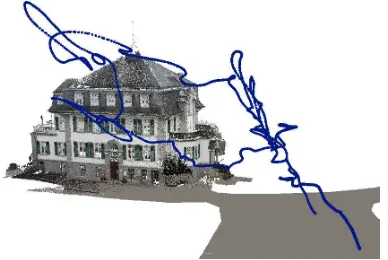
The first image sequence BUILDINGcontains 119 images taken with a 5 MPixel camera with a focal length ofc= 1587.87pixel on a 5 kg UAV platform, triggered each second. The flight was guiding the UAV along the facade of a house, the variation in position is around 60 m and 15 m in height, see Figure 2.
The second image sequence FIELD contains 24 images taken with a 12 MPixel camera of the DJI Panthom 4 with a focal length ofc = 2347.1pixel. The camera was pointing down-wards while the copter was flying a meandering pattern at 100 m height with three stripes, each stripe consists of eight images, see Figure 3. The images have an front and sidelap of 80 %, this way the 24 images cover an area of 100×90 m2
.
For both datasets we match interest points in the images to ob-tain corresponding image points. In order to determine the sim-plification effects, we need ground truth for camera poses and corresponding image points, to incorporate deteriorations under controlled conditions. We use the observed image coordinates as input for the BA softwareBACS(Schneider et al., 2012) to obtain estimated pose parameters and fitted image points for two real-istic UAV flight scenarios, which are consistent and are used as ground truth.
6.1 Checking the Rigorous Reference Solution
First we check how the rigorous trifocal BA reacts on differ-ent noise levelσ0lof observed image points on the BUILDING dataset. The estimated variance factorbσ2
0, see Eq. (19), needs to become one, in case the noise levelσ0lused to deteriorate the im-age points is used also in the covariance matrixΣallin Eq. (10). We follow Sec. 5.3 to generate deteriorated approximate values by using a moderate relative precision ofσ0x= 0.001. We deteri-orate the observations on each noise level 100 times with differ-ent random noise and apply the trifocal BA. Figure 4 shows the mean of the obtained standard deviationσ0b of estimated variance factors using different noise levelsσ0lto disturb the observed im-age points. Having high noise we observe, thatbσ0deviates from one, as then second order effects, which are neglected in the es-timation procedure of BA, become visible. The effects are negli-gibly small and within the tolerance bounds [0.9943, 1.0058] of
Figure 2. Trajectory of the UAV flight capturing the images of the BUILDINGdataset overlayed with a 3D model of a near-by
building.
Figure 3. Ground truth camera poses and 3D points of the FIELDdataset.
the fisher test using a significance level of 1 %. For the following evaluation of the accuracy decrease of the individual approxima-tions we will use a maximum noise level ofσ0l= 0.003.
Figure 5 shows the mean and standard deviation of the number of iterations until BA achieves convergence under different noise levels. The number of necessary iterations increases with the noise level as expected. Convergence is achieved if all corrections
noise level<0l[rad]
0 0.002 0.004 0.006 0.008 0.01
^
<0
1 1.0005 1.001 1.0015 1.002
Figure 4. The standard deviationbσ0of the estimated variance factor at different noise levelσ0l. With focal length c= 1587.87pixel, 0.001 radian corresponds to an uncertainty
of1.5pixel in the image points.
noise level<0l[rad]
0 0.002 0.004 0.006 0.008 0.01
n
u
m
b
er
of
it
er
at
io
n
s
0 2 4 6 8 10
Figure 5. The number of iterations needed to achieve convergence at different noise levelσ0land moderate relative precision ofσ0x= 0.001when usingTc= 0.001(blue line)
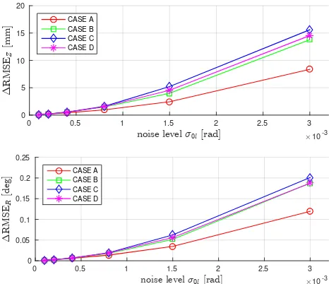
noise level<0l[rad] #10-3
Figure 6. Deviations between the RMSE of estimated camera positions and rotations of ideal result and approximations CASEA-D at different noise levelsσ0lof dataset BUILDING.
for observations∆lnc and parameters∆xuc are small compared to their standard deviation,|∆ln/σ0c l|< Tc,|∆xu/σxc u|< Tc,
with a thresholdTc= 0.001, thus requiring the corrections to be less than 0.1 % of their standard deviation. This requiresσxu to
be known, which is for this experiment derived in each iteration from the inverse normal equation matrix.
6.2 Effects of Approximations
We now experimentally evaluate the decrease of accuracy when applying the individual approximations for BA proposed in Sec. 5.2 on the two image sequences recorded by UAVs.
We add normal distributed noise to the true observation values with different magnitudes to obtain different noise levels. We use a moderate relative precision ofσ0x = 0.001to deteriorate the approximate values of the camera poses. After that we op-timize the pose parameters with the rigorous estimation, which is called CASE0 in the following, and with the approximations of CASEA-D. With the estimated and true pose parameters we can determine the root mean square error of the estimated camera positions and rotations according to Eq. (33) and Eq. (34). For each noise level we randomly generate 100 times different noise for the observations and determine the RMSE for each case. Fig-ure 6 and FigFig-ure 7 give the mean of the deviations of the RMSE of CASEA-D to the ideal result of CASE0 obtained with Eq. (35) under different noise levelsσ0l.
In both datasets the approximation made in CASEA induces the smallest deviations to the optimally estimated coordinates and ro-tations in both datasets, the deviations induced by the approxi-mation of CASEB are almost twice as big. CASEC, which con-tains the approximations of CASEA and CASEB, shows slightly higher deviations than CASEB, thus is mainly affected by the approximations of CASEB. CASED shows smaller deviations than CASEC, even though it contains an additional approxima-tion. The reason could be the high relative precisionσ0xused in this experiment. The convergence of CASED is affected by the relative precision as the weight matrixWggis fixed after the first
iteration, while CASEA-C are not affected. Thus we will inves-tigate the decrease in precision of CASED by varyingσ0x in a further experiment.
Figure 7. Deviations between the RMSE of estimated camera positions and rotations of ideal result and approximations CASEA-D at different noise levelsσ0lof dataset FIELD.
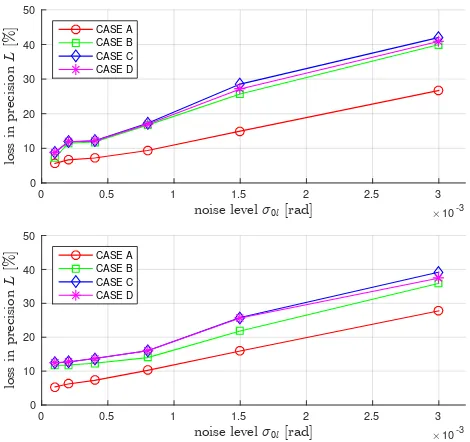
Figure 8 gives the loss in accuracyLCASE in percent, which can
be obtained with Eq. (36), under different noise levelσ0lfor each approximation. Both datasets recorded on different UAVs, flight trajectories and cameras show nearly the same loss in the accu-racy of the estimated poses due to the approximations.
The RMSE does not take the inhomogeneous uncertainty of the estimated positions and rotations of all images into account and depends on the chosen gauge. Thus we use the squared nor-malized Mahalanobis distance given in Eq. (37) which consid-ers the covariance information of the parametconsid-ers, which are ob-tained by the rigorous estimation. Table 1 lists the mean loss in accuracy∆FCASEof the estimated pose parameters in percent
when applying the individual approximation cases under differ-ent noise levelsσ0l. The loss of accuracy∆FCASE is obtained
with Eq. (38). The obtained values are similar to the values ob-tained by using the root mean square error.
CASEA, CASEB and therefore also CASEC are mainly affected by the noise levelσ0l, whereas CASED is affected from both, noise levelσ0land the relative precisionσ0xof the approximate values. Therefore we also investigate the average decrease in pre-cision by varyingσ0xfrom a moderate relative precision of 0.1 % to an inferior relative precision of 10 % to deteriorate the approx-imate values of the camera poses. We use a moderate noise level
σ0l= 0.0001 0.0002 0.0004 0.0008 0.0015 0.0030
BUILDING
CASEA 5.49 6.05 6.79 12.29 18.21 25.67 CASEB 9.87 11.34 11.73 14.75 21.90 36.92 CASEC 9.82 11.40 14.10 14.32 32.96 41.83 CASED 9.82 11.39 13.09 14.46 26.49 38.43
FIELD
CASEA 4.52 5.24 6.31 10.96 16.09 27.86 CASEB 11.36 11.45 11.21 12.76 20.86 33.03 CASEC 11.50 11.76 11.74 16.32 24.95 43.86 CASED 11.50 11.76 11.74 16.30 24.75 42.46
Table 1. The loss in accuracy∆FCASEin percent of estimated
noise level<0l[rad] #10-3
0 0.5 1 1.5 2 2.5 3
lo
ss
in
p
re
ci
si
on
L
[%
]
0 10 20 30 40 50
CASE A CASE B CASE C CASE D
noise level<0l[rad] #10-3
0 0.5 1 1.5 2 2.5 3
lo
ss
in
p
re
ci
si
on
L
[%
]
0 10 20 30 40 50
CASE A CASE B CASE C CASE D
Figure 8. The loss in accuracyLCASEin percent of
approximations CASEA-D compared to ideal solution at different noise levelsσ0lin radian on dataset BUILDING(top)
and FIELD(bottom).
ofσ0l= 0.001for the observations by adding normal distributed noise to the true observation values with different magnitudes to obtain different noise levels. Note that the estimated parameters converge differently when applying randomly generated approx-imate values. Thus, we randomly generate 100 times different noise for the observations and approximate values and determine the mean loss of accuracy∆FCASED for each relative precision levelσ0x. Table 2 shows the obtained∆FCASE, which increases
with the relative precisionσ0xof the approximate values for the camera poses.
In both experiments the decrease in accuracy is less than a 1/3 of noise variance. This is a moderate loss, and – if computing time is essential — may be accepted.
7. CONCLUSION
In this paper, we presented an approach to bundle adjustment without structure estimation by employing epipolar and trifocal constraints between corresponding image points. We introduced a novel closed-form expression for the trifocal constraint, which does not degenerate at certain configurations. The proposed bun-dle adjustment is as optimal as classical bunbun-dle adjustment, but leads to more computational complexity as the Gauss-Helmert model needs to be employed for optimization.
We evaluated the quality decrease of simplifying approximations which allow to employ the Gauss-Markov model to increase the
σ0x= 0.001 0.003 0.01 0.03 0.1
BUILDING
CASED 9.82 10.52 17.16 20.97 31.44 FIELD
CASED 11.50 13.28 14.52 16.94 25.36
Table 2. The loss in accuracy∆FCASEDin percent of estimated pose parameters at noise levelσ0l= 0.0001and different relative precisionσ0xof approximate values, both in radian.
computational efficiency on two datasets acquired by UAVs. The empirically investigated loss in accuracy of the estimated camera pose parameters are shown to be small in case of small noise in the observations.
In spite of this favorable result w.r.t. the investigated approxi-mations, the effect of the approximations onto outlier detection, which relies on the variances of the residuals needs to be investi-gated, in order to identify the loss in the power of outlier detection methods.
ACKNOWLEDGMENTS
This work has partly been supported by the DFG under the grant number FOR 1505: Mapping on Demand.
References
Agarwal, S., Furukawa, Y., Snavely, N., Simon, I., Curless, B., Seitz, S. and Szeliski, R., 2011. Building rome in a day. Com-munications of the ACM (CACM).
F¨orstner, W. and Wrobel, B., 2016. Photogrammetric Computer Vision – Statistics, Geometry, Orientation and Reconstruction. Springer.
Hartley, R. and Zisserman, A., 2004. Multiple View Geometry in Computer Vision. 2nd edn, Cambridge University Press.
Indelman, V., 2012. Bundle adjustment without iterative structure estimation and its application to navigation. In: Proc. of the Position Location and Navigation Symposium, pp. 748–756.
Indelman, V., Roberts, R., Beall, C. and Dellaert, F., 2012. In-cremental light bundle adjustment. In: Proc. of the British Machine Vision Conference, pp. 134.1–134.11.
Kaess, M., Johannsson, H., Roberts, R., Ila, V., Leonard, J. and Dellaert, F., 2012. iSAM2: Incremental Smoothing and Map-ping Using the Bayes Tree.Intl. Journal of Robotics Research (IJRR)31(2), pp. 217–236.
Konolige, K., 2010. Sparse sparse bundle adjustment. In:Proc. of the British Machine Vision Conference, pp. 102.1–102.11.
K¨ummerle, R., Grisetti, G., Strasdat, H., Konolige, K. and Bur-gard, W., 2011. G2o: A general framework for graph opti-mization. In: Proc. of the IEEE Intl. Conf. on Robotics & Automation (ICRA), pp. 3607–3613.
Lourakis, M. and Argyros, A., 2009. Sba: A software package for generic sparse bundle adjustment. ACM Trans. on Mathe-matical Software (TOMS)36(1), pp. 1–30.
Rodr´ıguez, A., de Teruel, P. L. and Ruiz, A., 2011. Reduced epipolar cost for accelerated incremental sfm. In: Proc. of the IEEE Conf. on Computer Vision and Pattern Recognition (CVPR), pp. 3097–3104.
Schneider, J., Schindler, F., L¨abe, T. and F¨orstner, W., 2012. Bun-dle adjustment for multi-camera systems with points at infinity. In:ISPRS Annals of the Photogrammetry, Remote Sensing and Spatial Information Sciences, Vol. I-3, pp. 75–80.
Stark, E. and Mikhail, E., 1973. Least Squares and Non-Linear Functions.Photogrammetric Engineering39, pp. 405–412.
Steffen, R., Frahm, J.-M. and F¨orstner, W., 2010. Relative bundle adjustment based on trifocal constraints. In:Trends and Top-ics in Computer Vision, Lecture Notes in Computer Science (LNCS), Vol. 6554, pp. 282–295.