MODELING A SPATIO-TEMPORAL INDIVIDUAL TRAVEL BEHAVIOR USING
GEOTAGGED SOCIAL NETWORK DATA: A CASE STUDY OF GREATER
CINCINNATI
M. Saeedimoghaddama, C. Kimb*1
aDepartment of Geography & GIS, University of Cincinnati, Cincinnati, OH 45221, United States, [email protected] bDepartment of Geography & GIS, University of Cincinnati, Cincinnati, OH 45221, United States, [email protected]
KEY WORDS: Spatiotemporal modeling, Location-based social network, Machine learning, Travel behavior
ABSTRACT:
Understanding individual travel behavior is vital in travel demand management as well as in urban and transportation planning. New data sources including mobile phone data and location-based social media (LBSM) data allow us to understand mobility behavior on an unprecedented level of details. Recent studies of trip purpose prediction tend to use machine learning (ML) methods, since they generally produce high levels of predictive accuracy. Few studies used LSBM as a large data source to extend its potential in predicting individual travel destination using ML techniques. In the presented research, we created a spatio-temporal probabilistic model based on an ensemble ML framework named “Random Forests” utilizing the travel extracted from geotagged Tweets in 419 census tracts of Greater Cincinnati area for predicting the tract ID of an individual’s travel destination at any time using the information of its origin. We evaluated the model accuracy using the travels extracted from the Tweets themselves as well as the travels from household travel survey. The Tweets and survey based travels that start from same tract in the south western parts of the study area is more likely to select same destination compare to the other parts. Also, both Tweets and survey based travels were affected by the attraction points in the downtown of Cincinnati and the tracts in the north eastern part of the area. Finally, both evaluations show that the model predictions are acceptable, but it cannot predict destination using inputs from other data sources as precise as the Tweets based data.
1. INTRODUCTION
With the evolution of urban travel demand models from aggregate to disaggregate models (Rasouli and Timmermans, 2014), there is a growing need of managing disaggregate travel data with spatial and temporal components in a GIS environment. Understanding travel behavior is vital in travel demand management as well as in urban and transportation planning (Yue et al., 2014; Beiró et al., 2016). Among the travel characteristics, trip destination and activity pattern received significant attention in recent studies (Ermagun et al., 2017). Traditionally, household travel survey sources are used to analysis human mobility pattern and travel behavior and create predictive models(Abbasi et al., 2015). The more recent studies tend to use machine learning (ML) methods since they generally produce higher levels of predictive accuracy than probabilistic and rule-based methods (Ermagun et al., 2017). (Deng and Ji, 2010) present a ML approach to deriving trip purpose from GPS track data coupled with other relevant data sources. They employ a number of attributes such as time stamp and land-use type of trip ends, a set of spatiotemporal indices of travel, and demographic and socioeconomic characteristics to construct a decision tree for purpose of classification. Similarly, (Lu et al., 2013) explore the feasibility of automating trip purpose detection employing ML method with geospatial location data, the land use data, and GPS-based survey data. (Oliveira et al., 2014) used a two-level nested logit model (probabilistic) and a decision tree model (ML) to differentiate between 12 trip purposes. In their study, the decision tree model was more accurate and much faster to generate functioning models than nested logit model. (Xiao et al., 2016) used artificial neural networks combined with particle swarm optimization to differentiate between 6 trip purposes from GPS data. To find the full list of previous studies in trip destination prediction, see (Lee et al., 2016; Ermagun et al., 2017).
*Corresponding author
New data sources including GPS logs, smart card records, mobile phone data, and location-based social media (LBSM) data (e.g.
Twitter, Foursquare, etc.) allow us to observe and understand mobility behavior on an unprecedented level of details and they have become potential alternatives or complementary approaches to study large-scale human mobility patterns and travel behaviors(Gao et al., 2014; Anda et al., 2017). LBSM data as a large volumes of spatio-temporal footprints (Li et al., 2013) can be specifically used in the predictive models of individual travel destination (Anda et al., 2017) based on ML techniques (Ermagun et al., 2017). Although GPS survey data was heavily utilized in predicting individual travel destination using ML methods, few studies used LBSM data as a big data source to extend its potential in this area. (Coffey and Pozdnoukhov, 2013) applied a ML method to enrich the semantics behind the modes related to the trip purpose and user activities at destinations in a bike sharing network using content-rich geo-referenced social media data. (Barchiesi et al., 2015) designed a ML algorithm to infer the probability of finding people in geographical locations and the probability of movement between pairs of locations using data from Flickr photo-sharing website. (Beiró et al., 2016) proposed a predictive model of human flow mobility that integrates a Flickr dataset with the classical gravity model, under a stacked regression procedure. They validated the performance and generalizability of the model using two ground-truth datasets on air travel and daily commuting in the United States.
offered in Section 2. Section 3 presents the modeling methodology and addresses the spatiotemporal specification of the ML model. Empirical results are presented in Section 4 along with an interpretation and validation. Section 5 concludes and offers thoughts for further research.
2. DATA & STUDY AREA
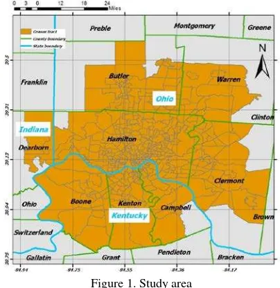
For this study, a Tweet crawler was developed based on the Twitter streaming API (application programming interface) to collect tweets posted within 419 census tracts of Greater Cincinnati area (Figure 1).
Figure 1. Study area
We collected 35 days of geotagged tweets between February 1, 2017 and March 11, 2017 and stored them in a spatial database. The dataset consists of over 46 thousand records generated by a total of over 4300 users. Each geo-tagged tweet has contents of the tweets and the associated exact location, timestamp and source, and also each Twitter user has a unique identifier and a profile name. Despite the 1% limit of sampling, it has been reported that the streaming API returns almost the complete set of the geo-tagged tweets (Morstatter et al., 2013). The extracted tweets are preprocessed before use for modeling because some i) geotagged-tweets are created by social-bots (Gao et al., 2014), ii) some tweets do not reflect the physical location of the user since the default location of the user saved in the location field instead, and iii) some users only create one tweet in the whole study time period making infeasible to create travel by only one tweet. After bot cleaning (Davis et al., 2016) 20360 (44% of total) geotagged tweets from 4188 users (96% of total) remained in the database. The mean inter-tweeting time was 232.02 minute (Figure 2).
Figure 2. Number of users for each mean inter-tweeting time
As the smartphone GPS uncertainty is typically up to 30 meters (Gao et al., 2014), we consider this number as the threshold for defining a trip. After the overall cleaning, 3529 travels from 560 users were created by considering each two consecutive tweets of a user in each day as a travel. Average number of trips per day was equal to 1 for 63%, 2 for 15%, 3 for 15%, 4 for 4% and more than 4 for 3% of the users (Figure 3).
Figure 3. Number of users for each average number of geo-tweets
Figure 4 shows the location of the tweets after cleaning and also the kernel density map of them. In addition to geotagged Tweets, The Household Travel Survey data provided by the Ohio-Kentucky-Indiana Regional Council of Governments (OKI) to explore the level of accuracy of the LBSM based model in predicting the destination of the trips extracted from other data sources. Between August 2009 and August 2010, the OKI Regional Council of Governments collected detailed travel data from 1137 households who carried around a Global Positioning System (GPS) handset tool when taking a trip. This survey recorded the trip information for each individual of every sampled household during weekdays, including trip purpose, origin locations, destination locations, transportation means, trip count, travel time, travel distance, and so on. In addition, this dataset also provides the socioeconomic and demographic information of each individual participating in the survey as well as the household information, such as gender, age, job type, income, household type and so on (Kim and Wang, 2015). Our final sample contains 6500 individuals located in the 419 census tracts.
Figure 4. Location of cleaned geo-tweets (top) and kernel density estimation (bottom)
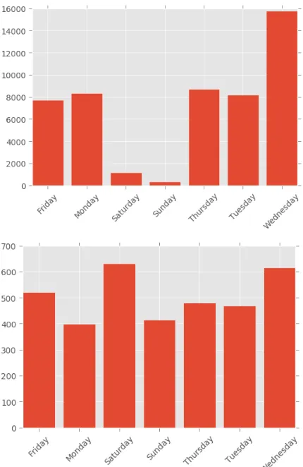
Figure 5. Number of travels in each week day based on survey data (top) and geo-tweets (bottom)
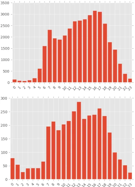
Figure 6. Number of travels in each hour of day based on survey data (top) and geo-tweets (bottom)
3. METHODOLOGY
3.1 Model Description
3.1.1 Random Forest model: Random forest (RF) model (Breiman, 2001) has demonstrated successful results in variety of travel behavior researches (Ermagun et al., 2017). We used this method to capture travel behavior in our study. RF is an ensemble learning approach where predictions are made based on multiple de-correlated decision trees built on training data using bootstrap aggregation or bagging procedure (Breiman, 1996). The procedure of creating a bagging predictor is resampling the training dataset with replacement, building a prediction model on each resampled dataset and averaging the prediction as in equation (1).
�����(�)(�) = 1�∑�=1� ��∗�(�) (1)
where ��(�) = predictor
X = features used as inputs of the function B = number of created bags of size n b = bag number.
Use of bagging in predictor leads to better model performance by decreasing the variance of the model, without increasing the bias. Using bagging in decision tree method can solve the overfitting problem of a single tree predictor because of the Law of Large Numbers (Breiman, 2001). According to the benefits of using bagging, RF method produces a large number of tree structures and uses all the trees to generate prediction results. It is also more stable than the individual decision tree models and less prone to errors in prediction due to data perturbations
(Ermagun et al., 2017). Figure 7 shows a flow chart for the modeling framework.
Figure 7. The flow chart of the modeling framework
of test data with unknown class and pj is the probability that each test data belongs to each class j of c, creating a probabilistic RF model for calculating pj consists of the following steps (John Lu, 2010):
Step 1. Draw a bootstrap sample Z* of size N from d train.
Step 2. Grow a random forest tree Tb for the bootstrapped data, by recursively repeating the following steps for each terminal node of the tree, until the minimum node size nmin is reached.
Step 2.1. Select m features at random from the q features of the data.
Step 2.2. Pick the best feature/split-point among them.
Step 2.3. Split the node into daughter nodes.
3.1.2 Calculation of the Model Parameters: For calculating pj for each test data, equation (1) is utilized by using Z* for B and N for n as the process of ensemble. In our study we used 5 features (q = 5) as the input of the model: i) census tract FIPS code of travel origin, ii) the landuse name where individual started his/her travel from there, iii) the time of the day, iv) the day of the week that the travel was started, and v) the population density of the origin census tract. The target classes (c) are the FIPS code of the census tract of individual destination. We used 80% of all travels of Twitter data as model’s training data (dtrain) and the remaining as test data (dtest) for model evaluation. For creating the forests, the following variables must be defined in the model: bootstrap sample size of dtrain (N), number of randomly selected features (m), the method for pick the best feature/split-point among the randomly selected features, maximum depth of each tree and the number of trees in each forest. Based on the size of the bootstrap sample, we control bias-variance tradeoff of random forest. It means that by choosing a large value for N we decrease the randomness and thus the forest is more likely to overfit. On the other hand, small value for N can reduce the degree of the overfitting at the expense of reducing the model performance. Choosing the number of samples in the original training dataset for N usually can provides a good bias-variance tradeoff (Phillips et al., 2016). We used this value for N in our study. For calculating the other variables of the model, k_fold cross validation method was used. k_fold divides all the samples in k groups, called folds. The prediction function is learned using k-1 folds, and the left out fold is used for test. the process is performed for each fold and based on the accuracy of each model the parameters of the highest accuracy will be considered as the optimum values (Kohavi, 1995). As 10-fold cross-validation is commonly used (McLachlan et al., 2005) we used 10 folds for optimizing the variables. After performing the optimization, the best value for i) the number of built trees in the forest was 700, ii) and m value was square root of the number of features (√5), iii) the depth of each tree was 9 and iv) “information gain” (IG) was used as the method for pick the best feature/split-point. IG is based on the notion of entropy, which characterizes the impurity of an arbitrary set of examples (Raileanu and Stoffel, 2004). Entropy of all the classes (ci) before splitting the data can be calculated by equation (2).
The expected entropy of attribute A with w distinct values after splitting the training data with A can be calculated by equation (3).
IG can be calculated using equation (4).
��(�) = � � �1
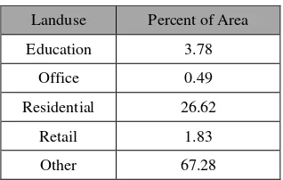
Best feature/split-point is the one with highest value of IG. In our study the number of classes (��) is 419 which is the number of census tract in the study area. The number of distinct value (w) for landuse attribute is 5 (Table 1), for days of the week is 7, for hours of a day is 5 as following: [0,5], [5,9], [9,12], [12,16], [16,24] (which are based on the hour categories of Census Transportation Planning Products (CTPP) (http://ctpp.transportation.org/)).
Landuse Percent of Area
Education 3.78
Office 0.49
Residential 26.62
Retail 1.83
Other 67.28
Table 1. Landuse composite in the study area
3.2 Model Evaluation
For evaluating the model performance, the area under the graph between the true positive and the false positive rates for the probabilistic classifier across all thresholds (ROC plot) was used. The resulting value varies between 0 and 1. 0.5 value shows that the model predicts randomly and values under 0.5 indicates that the model predicts the presence of an individual in a tract for which he/she was previously absent (Raven et al., 2002). The total AUC of the results was calculated using the method described in (Provost and Domingos, 2000). In this method, each AUC was weighted based on the prevalence of the tweets presence in a related class (Which is census tract in our research). The sum of the weighted values considered as the total AUC value. The procedure was performed for the household travel survey data and total AUC was calculated for it separately in order to examine the predictability of travel destinations using another data source which can be considered as an empirical evidence data.
4 EMPIRICAL RESULTS
data. Figure 8 shows the spatial distribution of AUC values calculated for each census tract for both Tweets based and survey based test data. The ‘None’ values show the tracts that were not predicted because they were not in the target column of the training data.
Figure 8. The spatial distribution of AUC values of Tweets based (top) and survey based (bottom) test data
As it can be noticed in Figure 8, several census tracts (about 33%) in Tweets based map have high values of AUC (0.8 to 1) but only 0.09% of the census tracts are in this range in the survey based map. The majority of AUC values (about 63%) in survey based map are in (0.6-0.7) range. Also 45% of the tracts have low value of AUC (0 to 0.5) in Tweets based map and about 28% of the tracts are in low value range. This huge number of tracts with low AUC value in Tweets based map does not make a low value of total AUC because model prediction was very accurate in the tracts with a lot of Tweet points. On the other hand, the total AUC value for survey based data is in accordance with the huge number of tracts with medium values of AUC in survey based map. There is no spatial pattern in the tracts with high AUC value in the Tweets based map however in survey based map as we move toward south western parts more tracts with high AUC can be seen. Based on this pattern it can be concluded
that the empirical based travels that starts from the south western parts have the same pattern in destination choosing with Tweet based travels that starts from the same regions.
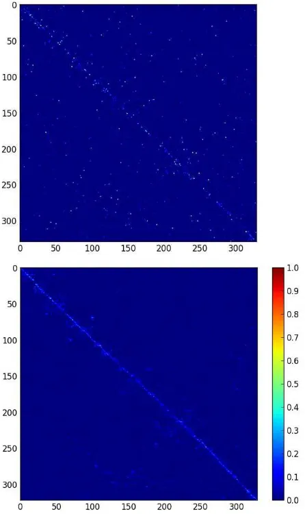
Comparing our study with some previous researches (Oliveira et al., 2014; Ermagun et al., 2017), our model seems to be more accurate. Our proposed approach can show useful information about the difference of the model predictions and the empirical pattern of destination choice. For example, Figure 9 shows the two rasters created from the OD matrices. The value of each cell was divided by the sum of its column in order to make the two rasters comparable to each other. The horizontal axis shows the destination tracts and the vertical axis shows the origin tracts. As it can be seen in Figure 9, the matrix of survey based travels is smoother than the model based one and majority of travels are on the main diagonal of the matrix which means there are a lot of intra tracts travels in this data and also it can be seen a recognizable spot in the down central part of the matrix. However, the model based raster has a distributed noisy pattern with non-dense main diagonal line which means model predicts a lot of inter travel between the tracts. Pearson correlation coefficient was 0.342 (p-value = 0.0001) showing a weak significant correlation between the matrices.
Figure 9. Raster of OD matrix created by all possible combination of model’s attributes (top) and the one created by
survey based travel data (bottom)
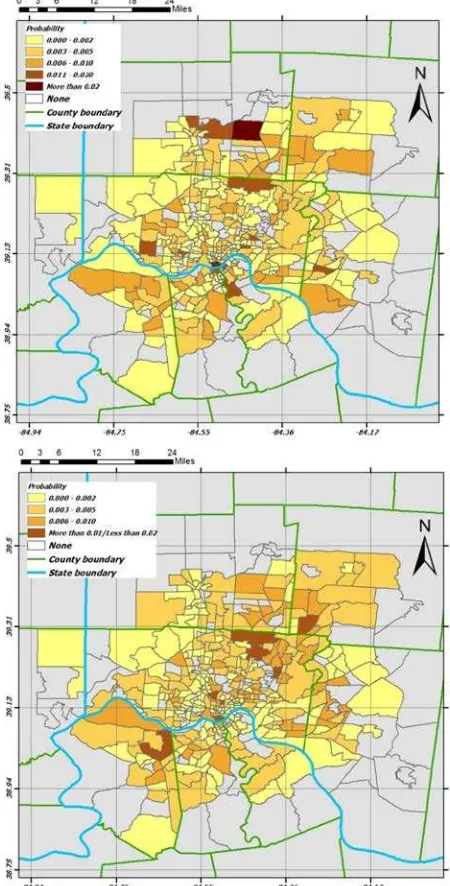
some tracts in downtown area of Cincinnati city and a tract in northern part have a high probability (more than 0.2) in the model based map. However, no tract in survey based map is in the high probability range. This fact is in proportion to the matrices pattern regarding to smooth pattern of the survey based matrix and noisy pattern of the model based one. The pattern of the model based map is affected by the number of Tweet travel destination points in each tract since the model is trained by Tweets data. Two spots of high values in the maps can be noticed. The first one is the downtown of Cincinnati city and the second one is two tracts in north eastern part of the area. The travel attraction of the downtown case was expected however the attraction of the other tracts was not. A possible reason for it, based on the location of the destination points inside of these two tracts, might be the existence of the shopping centers within them.
Figure 10. Probability of selecting each tract as the destination calculated by model based OD matrix (top) and survey based
OD matrix (bottom)
5 CONCLUSIONS & DISCUSSION
In this study, we created a probabilistic model to predict the destination of travels using RF (ML) method. Previous studies in travel destination estimation using ML method were typically based on GPS survey data. In this study we used geotagged Twitter data of 419 census tracts of Cincinnati metropolitan area in order to show its potential in modeling individual travel behavior. The accuracy of the model was acceptable for predicting the destination of the Tweet based travels. We concluded that the empirical based travels that starts from the south western parts of the study area is similar to destination choosing of Tweet based travels that starts from the same regions. In addition, both Tweets and survey based travels affected by the attraction points in the downtown area of Cincinnati and some tracts in the north eastern part of the area. Using LBSM data in travel behavior studies is effective because they allow us to observe and understand mobility behavior on an unprecedented level of detail. Although collecting this type of data is affordable compare to traditional surveys, there are couple of drawbacks when applying them to real world problems. First, the origin and destination of a travel created by LBSM are not specific places in many cases. For instance, they might be at the middle of roads and streets because some people tend to Tweet when they are in car. Furthermore, these data cannot be used in small study areas because the small number of samples might not represent the whole population. Because no exact demographic attributes exist in Tweet based travels, we extract them via external sources like landuse and census data. Thus our model is sensitive to the availability of these data. In this case, we could extract small amount of attributes for using in RF method and using more attributes might cause better results and accuracy. Further studies might be use of updated online data sources such as google maps (Ermagun et al., 2017) for extracting a more reliable landuse for origin and destination of the Tweet based travels. Another further study is using several sources of LBSM data such as Foursquare, Flicker, etc. in order to make a rich data source for modeling.
REFERENCES
Abbasi, A., Rashidi, T.H., Maghrebi, M., Waller, S.T., 2015. Utilising Location Based Social Media in Travel Survey Methods: bringing Twitter data into the play, ACM,Bellevue, WA, USA, pp. 1-9.
Anda, C., Erath, A., Fourie, P.J., 2017. Transport modelling in the age of big data. International Journal of Urban Sciences,
21, pp. 19-42.
Barchiesi, D., Preis, T., Bishop, S., Moat, H.S., 2015. Modelling human mobility patterns using photographic data shared online. Royal Society Open Science 2.
Beiró, M.G., Panisson, A., Tizzoni, M., Cattuto, C., 2016. Predicting human mobility through the assimilation of social media traces into mobility models. EPJ Data Science, 5, pp. 30.
Breiman, L., 1996. Bagging predictors. Machine Learning, 24, pp. 123-140.
Breiman, L., 2001. Random Forests. Machine Learning, 45, pp. 5-32.
Davis, C.A., Varol, O., Ferrara, E., Flammini, A., Menczer, F., 2016. BotOrNot: A System to Evaluate Social Bots,
International World Wide Web Conferences Steering Committee, Montréal, Québec, Canada, pp. 273-274.
Deng, Z., Ji, M., 2010. Deriving Rules for Trip Purpose Identification from GPS Travel Survey Data and Land Use Data: A Machine Learning Approach. Traffic and Transportation Studies 2010.
Ermagun, A., Fan, Y., Wolfson, J., Adomavicius, G., Das, K., 2017. Real-time trip purpose prediction using online location-based search and discovery services. Transportation Research
Part C: Emerging Technologies, 77, pp. 96-112.
Gao, S., Yang, J.-A., Yan, B., Hu, Y., Janowicz, K., McKenzie, G., 2014. Detecting origin-destination mobility flows from geotagged Tweets in greater Los Angeles area, Eighth International Conference on Geographic Information Science (GIScience'14).
Lu, Z., 2010. The elements of statistical learning: data mining, inference, and prediction. Journal of the Royal Statistical
Society: Series A (Statistics in Society), 173, pp. 693-694.
Kim, C., Wang, S., 2015. Empirical examination of
neighborhood context of individual travel behaviors. Applied
Geography, 60, pp. 230-239.
Kohavi, R., 1995. A study of cross-validation and bootstrap for
accuracy estimation and model selection, Ijcai. Stanford, CA,
1137-1145.
Lee, R.J., Sener, I.N., Mullins III, J.A., 2016. An evaluation of emerging data collection technologies for travel demand modeling: from research to practice. Transportation Letters, 8, pp. 181-193.
Li, L., Goodchild, M.F., Xu, B., 2013. Spatial, temporal, and socioeconomic patterns in the use of Twitter and Flickr.
Cartography and Geographic Information Science, 40, pp.
61-77.
Lu, Y., Zhu, S., Zhang, L., 2013. Imputing trip purpose based on GPS travel survey data and machine learning methods, Transportation Research Board 92nd Annual Meeting, Washington DC, USA.
Luo, F., Cao, G., Mulligan, K., Li, X., 2016. Explore spatiotemporal and demographic characteristics of human mobility via Twitter: A case study of Chicago. Applied Geography, 70, pp. 11-25.
McLachlan, G., Do, K.-A., Ambroise, C., 2005. Analyzing
microarray gene expression data. John Wiley & Sons, New
Jersey, USA, pp. 185-220.
Morstatter, F., Pfeffer, J., Liu, H., Carley, K.M., 2013. Is the Sample Good Enough? Comparing Data from Twitter's Streaming Api with Twitter's Firehose. In Proceedings of
ICWSM. Cambridge, MA: AAAI Press.
Oliveira, M., Vovsha, P., Wolf, J., Mitchell, M., 2014. Evaluation of Two Methods for Identifying Trip Purpose in GPS-Based Household Travel Surveys. Transportation
Research Record: Journal of the Transportation Research
Board, 2405, pp. 33-41.
Phillips, D., Romano, F., Czygan, M., Layton, R., Raschka, S., 2016. Python: Real-World Data Science. Packt Publishing Ltd, Birmingham, United Kingdom, pp. 63-96.
Provost, F., Domingos, P., 2000. Well-trained PETs: Improving probability estimation trees. CDER working paper #IS-00-04, Stern Shool of Business, NYU, NY, NY, 10012.
Raileanu, L.E., Stoffel, K., 2004. Theoretical Comparison between the Gini Index and Information Gain Criteria. Annals
of Mathematics and Artificial Intelligence, 41, pp. 77-93.
Rasouli, S., Timmermans, H., 2014. Activity-based models of travel demand: promises, progress and prospects. International
Journal of Urban Sciences, 18, pp. 31-60.
Raven, P.H., Scott, J.M., Heglund, P., Morrison, M.L., 2002.
Predicting Species Occurrences: Issues of Accuracy and Scale,
first ed. Island Press, Washington, D.C., pp. 303-314.
Xiao, G., Juan, Z., Zhang, C., 2016. Detecting trip purposes from smartphone-based travel surveys with artificial neural networks and particle swarm optimization. Transportation
Research Part C: Emerging Technologies, 71, pp. 447-463.
Yue, Y., Lan, T., Yeh, A.G., Li, Q.-Q., 2014. Zooming into individuals to understand the collective: A review of trajectory-based travel behaviour studies. Travel Behaviour and Society,