isprs archives XLII 4 W7 13 2017

(1)

A Comparison of Artificial Neural Network and Homotopy Continuation in 3D Interior Building

Modelling

Ali Jamali1, François Anton2, Alias Abdul Rahman1 and Darka Mioc2

1) Universiti Teknologi Malaysia (UTM) Faculty of Geoinformation and Real Estate

ali.jamali.65@gmail.com, alias@utm.my

2) Yachay Tech University School of Mathematics and Information Technology

fcastro@yachaytech.edu.ec, mioc@live.com

KEYWORDS: interval analysis, laser scanning, calibration, homotopy continuation, neural network, Levenberg–Marquardt algorithm

ABSTRACT:

Indoor surveying is currently based on laser scanning technology, which is time-consuming and costly. A construction model depends on complex calculations which need to manage a large number of measured points. This is suitable for the detailed geometrical models utilized for representation, yet excessively overstated when a simple model including walls, floors, roofs, entryways, and windows is required, such a basic model being a key for efficient network analysis such as shortest path finding. To reduce the time and cost of the indoor building data acquisition process, the Trimble LaserAce 1000 range finder is used. A comparison of neural network and a combined method of interval analysis and homotopy continuation in 3D interior building modelling for calibration of inaccurate surveying equipment is presented. We will present the interval valued homotopy model of the measurement of horizontal angles by the magnetometer component of the rangefinder. This model blends interval analysis and homotopy continuation. The results prove that homotopies give the best results both in terms of RMSE and the L_∞ metric.

1. INTRODUCTION

3D spatial modelling involves definition of spatial objects, data models, and attributes for visualization, interoperability and standards (Chen at al., 2008). Due to the complexity of the real world, 3D spatial modelling leads towards different approaches in different Geography Information Science (GIS) applications (Haala and Kada, 2010). In the last decade, there have been huge demands for 3D GIS due to the drastic advancement in the field of 3D computer graphics. According to Chen et al. (2008) there is not a universal 3D spatial model that can be used and shared between different applications, and different disciplines according to their input and output have used different spatial data models.

3D building modelling is an example of 3D spatial modelling. A building model has three spaces including a geometrical, a topological and a semantic space. This research focuses on the geometrical space. A topological model which is derived from a geometrical model defines relationships between connected and adjacent objects (e.g. rooms). A topological model is defined by a graph which is a navigable network consisting of nodes and edges. A semantic space presents attributes attached to geometrical and topological models.

According to Donath and Thurow (2007), considering various fields of applications for building modelling and various demands, geometry representation of a building is the

most crucial aspect of building modelling. For any kinds of emergency response, such as fire, smoke, and pollution, the interiors of the buildings need to be described along with the relative locations of the rooms, corridors, doors and exits as well as their relationships to adjacent spaces. The relationships between adjacent spaces need to be defined in a topological model.

Topological modelling is a challenging task in GIS environments, as the data structures required to express these relationships are particularly difficult to develop. To generate a topological model, a valid geometrical model is required. Indoor surveying is vital when no other data sources are available (e.g. there are no paper plans or architectural models). Unfortunately, many methods used for land surveying cannot be easily applied due to the lack of a GPS signal from satellites in indoor building environments, limited working areas inside buildings especially in office spaces, and very detailed environments with furniture and installations.

For many kinds of systems like disaster or emergency management systems, the interior models are essential (Boguslawski et al., 2011; Liu and Zlatanova, 2011). Indoor models can be reconstructed from construction plans, but sometimes they are not available or very often they differ

from ‘as-built’ plans. In this case, the buildings and its rooms must be surveyed. Perhaps, the most utilized method of

This contribution has been peer-reviewed.

https://doi.org/10.5194/isprs-archives-XLII-4-W7-13-2017 | © Authors 2017. CC BY 4.0 License.

(2)

indoor surveying is laser scanning. This method allows taking accurate and detailed measurements (Dongzhen et al., 2009; Yusuf, 2007).

This research intends to investigate complexity of interior building modelling and to demonstrate the feasibility of interior surveying. The proposed approach uses relatively

cheap equipment: a light ‘Laser Rangefinder’ which appears

to be the most feasible, but it needs to be tested to see if the observation accuracy is sufficient for the intended purpose: construction of a geometrical indoor building model.

However, any measurement device must be calibrated in order to control the uncertainties. The formal definition of calibration by the International Bureau of Weights and Measures (BIPM) is the following: "Operation that, under specified conditions, in a first step, establishes a relation between the quantity values with measurement uncertainties provided by measurement standards and corresponding indications with associated measurement uncertainties (of the calibrated instrument or secondary standard) and, in a second step, uses this information to establish a relation for obtaining a measurement result from an indication." (Clifford, 1985).

In this research, we provide a comparative analysis of 3D reconstruction and the indoor survey of a building using the Leica scanstation C10, the Trimble M3 and the Trimble LaserAce 1000 rangefinder. The Trimble LaserAce 1000 has been used for outdoor mapping and measurements, such as forestry measurement and GIS mapping (Jamali et al., 2013). A rangefinder can be considered as a basic mobile Total Station with limited functionality and low accuracy. The Trimble LaserAce 1000 is a three-dimensional laser rangefinder with point and shoot workflow. This rangefinder includes a pulsed laser distance meter and a compass, which can measure distance, horizontal angle and vertical angle up to 150 meters without a target, and up to 600 meters with a reflective foil target. The Trimble LaserAce 1000 will decrease the time and cost of the surveying process (Jamali et al., 2014).

The rangefinder has been used for forest applications by several researchers. Wing and Kellogg (2001) investigated the use of the laser rangefinder for harvest boundary measurement and skyline corridors. The laser rangefinder was used in traversing stand boundaries (Liu, 1995) and for estimation of wood piles volumes (Turcotte, 1999). The use of a laser rangefinder combined with GPS, total station and GIS for forest resources data collection and data mapping was investigated by Wing and Kellogg (2004).

Following this introduction, in Section 2, the data collection using a rangefinder is discussed. In Section 3, the rangefinder is calibrated using interval analysis and homotopy continuation in order to control the uncertainty of the calibration and of the reconstruction of the building. In Section 4, a neural network is used to minimize residual error

of the rangefinder. Section 5 presents conclusions and future research.

2. DATA COLLECTION

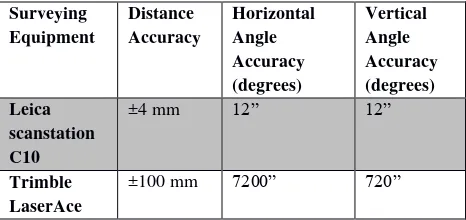
According to device specifications, the accuracies of the Leica scanstation C10, Trimble LaserAce 1000 are as shown in Table 1.

Table 1: Accuracies according to product specifications.

Surveying

To establish surveying benchmarks (control points), closed traverse surveying was used. Traverse surveying is a method of surveying for establishing control points along with traveling lines or movement paths. To get better results with less shape deformation (e.g. intersection and gap between two rooms due to low accuracy of Trimble LaserAce 1000), for each door, there should be a control point inside the corridor. For example, if a room has two doors, there should be two control points in the corridor to access that room by its two doors. There are 25 control points represented by Z1 to Z25 (see Figure 1), which represent the positions of the rangefinder inside the corridor or rooms. From the control points, slope distance, vertical angles and horizontal angles of top and down corners belonging to the room of interest will be measured (see Table 2).

Figure 1: Floor plan by Trimble LaserAce 1000.

Table 2: Measured slope distance (in meters), horizontal angles and vertical angles (in decimal degree) of top corners of room 1.

Room 1 point 1 point 2 point 3 point 4

slope distance 1 8.41 7.57 7.85 8.88

(3)

slope distance 2 8.4 7.58 7.85 8.87 slope distance 3 8.41 7.58 7.86 8.88 vertical angle 1 9.41 10.06 9.49 8.32 vertical angle 2 9.23 10.36 10 8.84 vertical angle 3 9.24 10.42 9.9 8.77 horizontal angle 1 268.4 336 99.6 166.1 horizontal angle 2 268.6 336.2 99.8 166.2 horizontal angle 3 269.1 335.9 99.9 166.5

Figure 2 shows the position of the rangefinder and measured points for room 1 (corners of the room 1).

Figure 2: Room 1, where the red point represents the position of the rangefinder and black points represent measured corners.

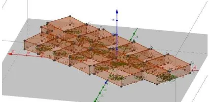
Coordinates measured by rangefinder are not as precise as a laser scanner or total station measurements. As seen in Figure 3, results of Trimble LaserAce 1000 show the deformation of building geometry.

Figure 3: 3D Building modelling by Trimble LaserAce 1000 where dashed lines represent measured data from Trimble LaserAce 1000 and solid lines represent extruded floor plan.

Figure 4 shows a 3D point cloud collected by the Leica scanstation C10.

Figure 4: Point cloud data collected by Leica scanstation C10.

Room 10 is our test case and room 1 is our reference (see Figure 5).

Figure 5: Room 10 as a normal case where the red point represents the position of the rangefinder and black points represent measured corners.

3. INTERVAL ANALYSIS AND HOMOTOPY CONTINUATION

In this section, we will present our interval valued homotopy model of the measurement of horizontal angles by the magnetometer component of the rangefinder. This model blends interval analysis and homotopy continuation. Interval analysis is a well-known method for computing bounds of a function, being given bounds on the variables of that function (Moore and Cloud, 2009). The basic mathematical object in interval analysis is the interval instead of the variable. The operators need to be redefined to operate on intervals instead of real variables. This leads to interval arithmetic. In the same way, most usual mathematical functions are redefined by an interval equivalent. Interval analysis allows one to certify computations on intervals by providing bounds on the results. The uncertainty of each measure can be represented using an interval defined either by a lower bound and a higher bound or a midpoint value and a radius.

In this paper, we use interval analysis to model the uncertainty of each measurement of horizontal angle and

(4)

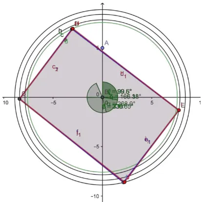
horizontal distance done by the rangefinder. We represent the geometric loci corresponding to each surveyed point as functions of the bounds of each measurement. Thus, for distances observed from a position of the rangefinder, we represent the possible position of the surveyed point by two concentric circles centered on the position of the rangefinder and of radii the measured distance plus and minus the uncertainty on the distance respectively (see Figure 6). For horizontal angles observed from a position of the rangefinder, we represent the possible position of the surveyed point by two rays emanating from the position of the rangefinder and whose angles with respect to a given point or the north are the measured angle plus and minus the uncertainty on the horizontal angle, respectively (see Figure 6). Therefore, the surveyed point must be within a region bounded by these four loci: in between two concentric circles and two rays. Proceeding in the same way for each room, we get the geometric loci for each room and for the union of the surveyed rooms (see Figure 7).

A homotopy is a continuous deformation of geometric figures or paths or more generally, functions: a function (or a path, or a geometric figure) is continuously deformed into another one (Allgower and Georg, 1990). A homotopy between two continuous functions f0 and f1 from a topological space X to a topological space Y is defined as a

continuous map H: X × [0, 1] → Y from the Cartesian

product of the topological space X with the unit interval [0, 1] to Y such that H(x, 0) = f0, and H(x, 1) = f1, where x ∈ X. The two functions f0 and f1 are called, respectively, the initial and terminal maps. The second parameter of H, also called the homotopy parameter, allows for a continuous deformation of f0 to f1 (Allgower and Georg, 1990). Two continuous functions f0 and f1 are said to be homotopic, denoted by f0≃ f1, if and only if there is a homotopy H taking f0 to f1. Being homotopic is an equivalence relation on the set C(X, Y) of all continuous functions from X to Y.

Figure 6: The geometric loci of one corner of a room as a function of its related measurements.

Figure 7: The geometric loci of each corner of a room as a function of all the measurements.

Figure 8: The reconstruction of Room 1 from original rangefinder measurements (red) and interval valued homotopy continuation calibration of horizontal angles measurements (blue).

In this paper, we used homotopy to calibrate the rangefinder. The main idea is that the 360 degrees compass of the magnetometer is subject to continuous deformations, which do not induce any cut of any single part of this compass, nor any gluing of different parts of this compass. We can therefore think that the 360 degrees compass of the magnetometer is made of a highly deformable material like plastic, while the 360 degrees compass of the theodolite component of a total station is made of a very non-deformable material like temperature invariant metal. The alteration of the magnetic field of the Earth when, for example, a truck is passing near the range finder, can be modeled as an elastic continuous deformation of the 360 degrees compass of the magnetometer. Unlike in the previous methodologies, we only assume that the calibration of the set of our rangefinder measurements with respect to the set of measurements of our total station can be done continuously, because there is no discontinuity in the n-dimensional space corresponding to the space of measurements performed using the rangefinder and the total station. Even though not all real numbers are representable in a digital measurement device,

(5)

we can assume that all the real numbers corresponding to measurements can be obtained physically, and it is just the fixed point notation used by the digital measurement device that limits the set of representable real numbers to a discrete subset of the set of real numbers. Thus, we can compute the calibration of the rangefinder as a continuous function mapping our measurements obtained using our rangefinder to the measurements obtained using our total station, corresponding to the inverse elastic transformation from the flexible magnetometer 360 degrees compass to the rigid 360 degrees compass of the theodolite component of the total station.

The results of the linear homotopy continuation are shown in Figure 8 and Tables 3–5. One can calibrate the differences of horizontal angles observed with the rangefinder to the differences of horizontal angles observed with the theodolite. One can start from any point and assume that the horizontal angles made with the rangefinder. We calibrate the new measurements of horizontal angles made by the rangefinder in each one of these intervals as a non-linear homotopy, where the homotopy parameter is the relative position of the measured horizontal angle in between the bounds of the enclosing interval of rangefinder horizontal angles. This homotopy calibration can be visualized as the continuous deformation of each sector (defined by the rangefinder horizontal angle intervals of room 1) of a plastic

disk (corresponding to the old time theodolite graduated disk) to the corresponding sector of the total station’s theodolite graduated disk. We used the intervals of total station horizontal angles of room 1 as reference intervals for all other horizontal angle measurements in rooms 1and 10.

In the remainder of the paper, “the homotopy parameter of a

horizontal angle measurement” is equivalent to “the relative

position of the horizontal angle measurement in the

corresponding reference interval.” We fitted a polynomial of

degree 5 through the four points whose x-coordinates are the homotopy parameters of the horizontal angles measured by the rangefinder in room 10 and the corresponding homotopy parameters of the horizontal angles measured by the total station in room 10 and the points (0,0) and (1,1). We used this polynomial as the convex homotopy function that maps the uncalibrated homotopy parameter to the calibrated one.

The initial and terminal maps correspond respectively to the mappings between the uncalibrated and calibrated horizontal angles at the start point and the end point of the enclosing interval of horizontal angles measured by the rangefinder. We can see that, contrary to the least squares calibration, the only limitation of this interval analysis and homotopy continuation-based calibration is the precision of the fixed point arithmetic used by the computing device used for the calibration.

Table 3: Calibration of room 1 rangefinder horizontal angle measurements by homotopies (in decimal degrees).

Point Rangefinder

2 336.0 67.745139 336.645139 122.85028 122.85028

3 99.6 190.595419 99.495417 65.881667 65.881667

4 166.1 256.477086 165.377083 294.264583 294.264583

5 98.5 190.741669 99.641667 169.258333 169.258333

Table 4: Calibration of room 10 rangefinder horizontal angle measurements by homotopies (in decimal degrees).

Point Horizontal angle

(6)

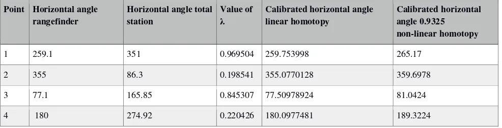
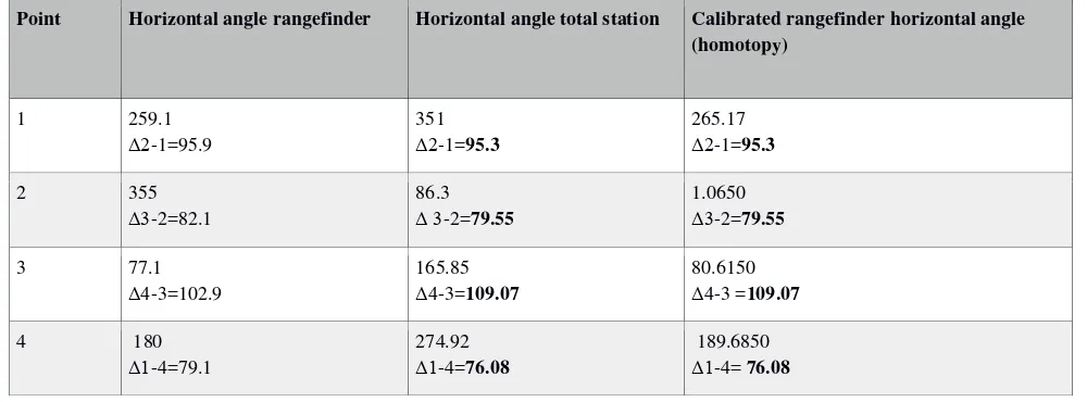
Table 5: Calibration of room 10 rangefinder horizontal angle measurements using total station horizontal angle measurements by homotopies (in decimal degrees).

Point Horizontal angle rangefinder Horizontal angle total station Calibrated rangefinder horizontal angle (homotopy)

1 259.1

Δ2-1=95.9

351

Δ2-1=95.3

265.17

Δ2-1=95.3

2 355

Δ3-2=82.1

86.3

Δ 3-2=79.55

1.0650

Δ3-2=79.55

3 77.1

Δ4-3=102.9

165.85

Δ4-3=109.07

80.6150

Δ4-3 =109.07

4 180

Δ1-4=79.1

274.92

Δ1-4=76.08

189.6850

Δ1-4= 76.08

4. NEURAL NETWORK

In this section, we used neural network (Gevrey et al., 2003) to minimize residual errors of the rangefinder measurement using Total Station measurement. An artificial neural network is designed by several interconnected nodes which are called neurons. In an artificial neural network, there can be three layers including input, hidden and output layer (see Figure 9). To train the artificial neural network, data is required to be divided into three datasets as training, validation and test data. Input data are the rangefinder measurements and target data are Total Station data. The best way to determine the most suitable number of hidden neurons is to train several networks. Few number of hidden neurons result in a higher total error and on the other hand, too many hidden neurons results in an over-fit function with an increased validation error.

Figure 9: An artificial neural network architecture.

Our training algorithm is Levenberg-Marquardt (Levenberg, 1944; Marquardt, 1963; Moré, 1978; Lourakis, 2005). Levenberg-Marquardt algorithm is an iterative technique that determines the minimum of a multivariate function that is presented as the sum of squares of non-linear real-valued functions. It is a standard technique for non-linear least-squares problems (Lourakis, 2005) (see Equation 1). This experiment has been done by Matlab neural network toolbox.

�+ = �− �� + � − � �

Where µ is always positive, called combination coefficient, k is the index of iterations,

w is the weight vector, e is error vector,

J is the Jacobian matrix that contains first derivatives of the network errors with respect to the weights and biases, And I is the identity matrix.

When the scalar µ is near zero, Gauss-Newton's method is used (see Equation 3). When µ is big, steepest descent method is used (see Equation 2). If the error (see Equation 4) is decreasing, which means that it is smaller than the last error; it indicates that the quadratic approximation on total

error function is working and the combination coefficient μ is

required to be decreased to reduce the influence of gradient descent part. If the error is increasing, which means it is

larger than the last error; the combination coefficient μ is

required to be increased (Yu and Wilamowski, 2011).

(7)

�+ = �−∝ ��

�+ = �− �� − � �

g is gradient vector,

α is the learning constant (step size),

� , = . ∑ ∑ �,

= �

�=

Where x is input vector,

w is the weight vector,

ep,m is the training error at output m when applying pattern p (see Equation 5).

�, = �, − ��,

Where d is the desired output vector,

o is the actual output vector.

Training process using Levenberg-Marquardt algorithm is explained as follows (see Figure 10):

i. With initial weights which are randomly generated, total error (see Equation 7) is evaluated.

ii. Equation 4 is used to update the weights. iii. Total error is evaluated with the new weights. iv. If total error is increased then we need to go back

one step before and use previous weights. µ value is required to be increased as well. We need to move to step 2.

v. If total error is decreased, we accept the update and we need to decrease µ value by the same factor used in step 4.

vi. We need to move to step 2. Process continues till the total error is smaller than the desired total error value (Yu and Wilamowski, 2011).

Figure 10: Block diagram for training using Levenberg– Marquardt algorithm: wk is the current weight, wk+1 is the

next weight, E k+1 is the current total error, and Ek is the last total error (Yu and Wilamowski, 2011).

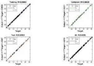
We used 70 percent of our total data for training, 15 percent for validation and 15 percent for test with 10 neurons as the hidden layer. The four plots represent the training, validation, testing, and all data. The targets are represented by the dashed line in each plot. The best fit linear regression line between outputs and targets is represented by the solid line. The R value represents the correlation between the outputs and targets. If R = 1, this means that there is an exact linear correlation between outputs and targets. If R is close to zero, then there is no linear correlation between outputs and targets. In our experiment, the training data shows a good fit. The validation and test results also represent R values that are greater than 0.9. The scatter plot is useful when certain data points have poor fits (see Figure 11).

Figure 11: The training, validation, testing data, and all data plots.

We have minimum number of results with residual errors of higher than 1 meter and maximum number of results with residual error of less than 0.1 meter (see Figure 12).

Figure 12: Error histogram where blue color represents training data, green color represents validation data and red

color represents test data.

The best validation performance for error goal is 0.19733 meter in iteration 21 (see Figure 13).

(8)

Figure 13: Performance histogram where blue line represents train data, green line represents validation data and red line

represents test data.

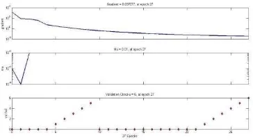
Gradient is equal to 0.037077 at iteration 27 and µ is equal to 0.01 at iteration 27 (see Figure 14).

Figure 14: The gradient, µ values and validation checks.

Geometrical information using neural network and homotopy continuation for room 10 is presented in Table 7.

Table 7: Calibration of room 10 rangefinder horizontal angle measurements using total station horizontal angle measurements by homotopies and neural network (in decimal degrees).

Point Horizontal angle rangefinder

Horizontal angle total station

Calibrated rangefinder horizontal angle (homotopy)

Calibrated rangefinder horizontal angle (neural network)

Δ2-1 95.9 95.3 95.3 96.08

Δ3-2 82.1 79.55 79.55 82.07

Δ4-3 102.9 109.07 109.07 100.57

Δ1-4 79.1 76.08 76.08 81.27

The results shown in Table 7 prove that homotopies give the best results both in terms of RMSE and the L_∞ metric (which corresponds to the maximum among all components of the input vector �_∞ = �� ⁡{ , ⋯ , } as can be read in (Rudin, 1980).

5. CONCLUSIONS

Rangefinder data was calibrated by neural network, which shows a maximum residual error of 8.5 degree and a minimum residual error of 0.78 degree in room 10 using neural network. However, the combined interval analysis and homotopy continuation technique calibration obtained by continuous deformation of the function mapping, the rangefinder measurements to the theodolite measurements allows a much better match, whose only limitation is the fixed point arithmetic of the computing device used to perform the computation. For room 10 using homotopy continuations, we have a residual error of 0 degree (see Table 7). Our research group will investigate a topological

mathematical indoor model reconstruction based on the homotopy continuation in the near future.

REFERENCES

Allgower, E. L., & K. Georg, (1990). Numerical continuation methods: an introduction. Springer-Verlag New York, Inc. New York, NY, USA.

Chen, T.K., Abdul-Rahmana, A. &Zlatanova, S., (2008). 3D Spatial Operations for geo-DBMS: geometry vs. topology. The International Archives of the Photogrammetry, Remote Sensing and Spatial Information Sciences, XXXVII(B2): 549-554.

Deak, G., Curran, K., & Condell, J. (2012).A survey of active and passive indoor localisation systems. Computer Communications, 35(16), 1939–1954.

Donath, D., &Thurow, T. (2007).Integrated architectural surveying and planning. Automation in Construction, 16(1), 19–27.

(9)

Dongzhen, J., Khoon, T., Zheng, Z., & Qi, Z. (2009). Indoor 3D Modeling and Visualization with a 3D Terrestrial Laser Scanner. 3D Geo-Information Sciences, 247–255.

Gevrey, M., Dimopoulos, I., &Lek, S. (2003). Review and comparison of methods to study the contribution of variables in artificial neural network models.Ecological modelling, 160(3), 249-264.

Haala, N., &Kada, M. (2010).An update on automatic 3D building reconstruction. ISPRS Journal of Photogrammetry and Remote Sensing, 65(6), 570–580.

Jamali, A., Boguslawski, P., Duncan, E. E., Gold, C. M., & Rahman, A. A. (2013).Rapid Indoor Data Acquisition for Ladm-Based 3d Cadastre Model. ISPRS Annals of Photogrammetry, Remote Sensing and Spatial Information Sciences, 1(1), 153-156.

Jamali, A., Boguslawski, P., Gold, C. M., & Rahman, A. A. (2014).Rapid Indoor Data Acquisition Technique for Indoor Building Surveying for Cadastre Application.In Innovations in 3D Geo-Information Sciences (pp. 1-11).Springer International Publishing.

Jamali, A., Rahman, A. A., Boguslawski, P., Kumar, P., & Gold, C. M. (2017). An automated 3D modeling of topological indoor navigation network. GeoJournal, 82(1), 157-170.

Kim, J. S., Yoo, S. J., & Li, K. J. (2014).Integrating IndoorGML and CityGML for Indoor Space. In Web and Wireless Geographical Information Systems (pp. 184-196). Springer Berlin Heidelberg.

Levenberg, K. (1944). A method for the solution of certain non-linear problems in least squares.Quarterly of applied mathematics, 2(2), 164-168.

Li, K. J., & Lee, J. Y. (2013).Basic concepts of indoor spatial information candidate standard IndoorGML and its applications.Journal of Korea Spatial Information Society, 21(3), 1-10.

Liu, L., &Zlatanova, S. (2011). Towards a 3D network model for indoor navigation.Urban and Regional Data Management, UDMS Annual, 79-92.

Lourakis, M. I. (2005). A brief description of the Levenberg-Marquardt algorithm implemented by levmar.Foundation of Research and Technology, 4(1).

Luo, F., Cao, G., & Li, X. (2014, November). An interactive approach for deriving geometric network models in 3D

indoor environments. In Proceedings of the Sixth ACM SIGSPATIAL International Workshop on Indoor Spatial Awareness (pp. 9-16).ACM.

Marquardt, D. W. (1963). An algorithm for least-squares estimation of nonlinear parameters.Journal of the society for Industrial and Applied Mathematics, 11(2), 431-441.

Moré, J. J. (1978). The Levenberg-Marquardt algorithm: implementation and theory. In Numerical analysis (pp. 105-116).Springer Berlin Heidelberg.

Ramon Moore, R. K. E., & Cloud, M. J. (2009).Introduction to interval analysis. SIAM (Society for Industrial and Applied Mathematics), Philadelphia.

Rudin, Walter (1980), Real and Complex Analysis (2nd ed.), New Delhi: Tata McGraw-Hill, ISBN 9780070542341.

Tang, P., Huber, D., Akinci, B., Lipman, R., & Lytle, A. (2010). Automatic reconstruction of as-built building information models from laser-scanned point clouds: A review of related techniques. Automation in construction, 19(7), 829-843.

Teo, T. A., & Cho, K. H. (2016).BIM-oriented indoor network model for indoor and outdoor combined route planning.Advanced Engineering Informatics, 30(3), 268-282.

Turcotte, P. (1999). The Use of a Laser Rangefinder for Measuring Wood Piles.Forest Engineering Institute of Canada Field Note 76, Pointe Claire, Quebec, Canada.2 p.

Volk, R., Stengel, J., &Schultmann, F. (2014). Building Information Modeling (BIM) for existing buildings— Literature review and future needs. Automation in construction, 38, 109-127.

Wing, M., & Kellogg, L. (2001, June). Using a laser range finder to assist harvest planning.In Proceedings of the First International Precision Forestry Cooperative Symposium, Seattle, WA, USA (pp. 147-150).

Wing, M. G., & Kellogg, L. D. (2004, June).Digital data collection and analysis techniques for forestry applications.In Proceedings of the12th International Conference on Geoinformatics, University of Gävle, Sweden (pp. 77-83).

Yu, H., &Wilamowski, B. M. (2011).Levenberg–marquardt training.Industrial Electronics Handbook, 5(12), 1.

Yusuf, A. (2007). An approach for real world data modeling with the 3D terrestrial laser scanner for built environment. Automation in Construction, 16(6): 816-829.