Lionardus Ruslim Deddy Marciano Liliana Inggrit

(1)

The Test of IPO’s Underpricing Between Financial and Non Financial Institution Based on

Asymmetric Information Hyphothesis

Lionardus Ruslim1 Deddy Marciano2 Liliana Inggrit Wijaya3

Abstract

This research aims to prove underpricing IPO differences between financial institution and non-financial institution during 2001-2008 period. In addition, this research also examined the causes of underpricing IPO ’s of financial institution and nonfinancial institution using asymmetric information hypothesis. This research uses initial return and abnormal return as a measure to know which one is better as an underpricing measurement. Furthermore, the calculation in this research is using the open to close prices data to have more accurate results and not biased.

The tests are using one sample t-test, independent t-test, and the ordinary least square regression to analyze the data. One sample t-test is used to prove occurrence of institutions’s underpricing at observation period. Independent t-test is used to determine differences significance in underpricing. Whereas, ordinary least square regression to determine the causes of underpricing. Each test uses an initial return and abnormal return as a measure.

This research found that IPOs are significantly underpriced at the first day of trading. Financial institutions sector’s IPOs are less underpriced than non-financial institutions sectors. This findings means that financial institution sector have less asymmetric information than non-financial institution sectors. This study concludes that the regulation and the monitoring for the financial institution sector have developed better than the previous few years. In addition, there are several factors that affect underpricing. These factors are the type of business entities and trade price volatility in the stock market. The usage of both initial return and abnormal return to measure underpricing level are not significantly different. Furthermore, usage of open to close price data is able to give more accurate results for calculations to measure underpricing level.

Keywords:underpricing, asymmetric information, regulation hypothesis, initial return, abnormal return

---1 Lionardus Ruslim, S.E., RFPI.: Alumnus Faculty of Business and Economics University of Surabaya. (leeyo13@gmail.com) 2 Dr. Deddy Marciano, S.E., M.M. : Researcher of Center for Business & Industrial Studies (CBIS) and Lecturer of Faculty of

Business and Economics University of Surabaya

3 Drs. ec. Liiana Inggrit Wijaya, M.M., RFPI., CFP., AEPP. : Chair of Master of Management Programme and Lecturer of Faculty of Business and Economics University of Surabaya

I. Introduction

Growing firms have several options to fund their expansion of operational activities. One of the options in financing enterprise operational processes is going public. Activities of firms that sell shares first time to public called the Initial Public Offering (IPO). One of the important stages in the IPO process is determining underwriters who have a good reputation (see Ruud, 1993; Alli et al, 1994; Ernyan and Husnan, 1997; Triaryati and Husnan, 2004).

(2)

often seemed in the IPO.

This research aims to tell the difference underpricing that happen between regulated firms (financial institutions) and non regulated firms. Underpricing differences between the financial institutions and non-financial institutions may happen because of differences in information asymmetry in the financial institutions and non-financial institutions. The study also aims to test several factors that affect underpricing of IPO’ s. These factors are type of institutions, risk (standard deviation), underwriter reputation, and age of institution. We expect that these factors can explain the underpricing of IPO’s.

Several previous studies are using the initial return (Alli et al, 1994; Ernyan and Husnan, 1997) and abnormal return (Triaryati and Husnan; 2004) as a measure to determine the level of underpricing. This research will use both types of measurements to know which measurements are better for explaining asymmetric information. We use open to close price data for calculation to measure underpricing level. This is necessary in order to obtain research results that are unbiased and more accurate. Previous studies using close to close price data as the reference calculation underpricing. This can lead to bias result due to the closing price today are not always become the opening price the next trading day. For investors who want to buy the securities by reference to the closing price the previous day, may not be able to purchase that securities because of possible changes on the opening price the next day.

II. Literature Review

Generally, underpricing occurs when the IPO price is cheaper than prices in the secondary market on the first day of trading, allowing investors to get an abnormal return. Ruud (1993) said “Over the past two decades, several empirical studies have reported that initial public offerings sizeable achieve average returns over very short periods, suggesting that the offerings may be underpriced”. Ross et al (2005:548) said that there are two facts found on the underpricing puzzle. First, many of underpricing is concentrated in less offerings. Second, when the bid price is too cheap, the demand of IPO is often oversubscribed. To identify the occurrence of IPO underpricing in Indonesian Capital Market, the first hypothesis is that there is underpricing occurred on the first day of trading after IPO. The first hypothesis would be divided to two minor hypotheses. Hypothesis 1a is that there is positive average initial return on the first day of trading after IPO. While 1b hypothesis is that there is a positive average abnormal return on the first day of trading after IPO.

Asymmetric information is the difference of information happened between the parties involved in the IPO, the underwriters, business entities, and potential investors (Ernyan and Husnan, 1997). Underwriters have more complete information about the market than the firms. Furthermore underwriters have more information about firms rather than potential investors. As a result, there was a difference of information held by businesses on market conditions, and potential investors about the condition of the firms. The greater the information asymmetry faced by potential investors, the greater they penalized the price of primary market. This (penalty done by investors) will force underwriters to offer these shares at a low price (underpriced).

Regulation hypothesis explains that government regulations are applied to reduce the asymmetric information between the management with outsiders, including potential investors. So the underpricing of regulated firms will be less than non-regulated firms. Alli et al (1994) find that underpricing is happening in the financial instituitions are less than non-financial institutions. Thus, hypothesis two is underpricing of financial institutions will be less than non-financial institutions. This hypothesis would be divided to two minor hypotheses. Hypothesis 2a is the initial return on the financial institutions are less than non-financial institutions. Whereas hypothesis 2b is the abnormal return on the financial institutions are less than non-financial institutions.

(3)

financial institutions is less than non-financial institutions. The next hypothesis is hypothesis 4, the risk have a positive effect on underpricing of IPO. Hypothesis 4 also will be divided to two minor hypotheses. Hypothesis 4a is standard deviation has positive effect on initial return. Hypothesis 4b is, standard deviation has positive effect on abnormal return. Furthermore, ex-ante uncertainty is also related to the reverse of gross proceed (prime stocks capitalization). The less the values of reverse gross proceed will reduce investor speculation on the stock. So the value of reverse gross proceed will goes to the opposite direction to the level of underpricing.

Maurer and Senbet (1992) in Triaryati and Husnan (2004) showed that the age of the firms has negative effect on initial return. So, the older the firm establish, the lower underpricing level will be occurred. Hypothesis 5 is the age of firms has negative effect on underpricing of IPO. Hypothesis 5 will be divided into two minor hypotheses. Hypothesis 5a is age of the firms has negative effect the initial return on the IPO. Hypothesis 5b is age of the firms has negative effect the abnormal return on the IPO.

Michaely and Shaw (1994) said that the better the reputation of underwriters, the lower the initial return occurs on IPO. Related to this statement, Triaryati and Husnan (2004) explained that reputable underwriters will tend to avoid risky IPO emission because it can threatening their reputation and sustainability. To measure reputation of the underwriters, we use ratio of the market share of each underwriter who perform underwriting the IPO to the total market share the underwriters as a proxy. Hypothesis 6 is the reputation of underwriters has negative effect on underpricing of IPO. Hypothesis 6 will be divided to two minor hypotheses. Hypothesis 6a is underwriter market share has a negative effect on the initial return. Hypothesis 6b is the underwriter market share has negative effect on the abnormal return.

III. Research Method and Data

This study uses data obtained from financial laboratory databases FBE-UBAYA, yahoo finance website, IDX website, and IMQ Antara website. These sources provide all of IPOs that made from 2001-2008 period, date of the IPO, date of the firm established, industries and sub-industries, main underwriters for each IPO, number of shares offered, opening and closing price for 20 days trading after the IPO, value of the opening and closing Composite Stock Price Index for 20 day trading adjusted for each firms.

Table 1

RESEARCH POPULATION (2001-2008)

Financial Institutions

Bank Non-Bank Total

Non-Financial Institutions

Year _Σ_IPO _% _Σ_IPO _% _Σ_IPO _% _Σ_IPO _%

2001 2 14.29 2 13.33 4 13.79 15 18.99

2002 3 21.43 3 20.00 6 20.69 11 13.92

2003 2 14.29 1 6.67 3 10.34 2 2.53

2004 0 0.00 4 26.67 4 13.79 8 10.13

2005 0 0.00 4 26.67 4 13.79 3 3.80

2006 3 21.43 0 0.00 3 10.34 8 10.13

2007 3 21.43 0 0.00 3 10.34 18 22.78

2008 1 7.14 1 6.67 2 6.90 14 17.72

Total 14 100.00 15 100.00 29 100.00 79 100.00

Sources:Indonesian Stock Exchange and Financial Laboratory Database FBE UBAYA

We use initial return and abnormal return as a measurement to indicate level of underpricing. Initial return is the return obtained from the time purchased in the primary market to be listed first in the secondary market (Jogiyanto, 2008:33). To avoid bias due to the influence of divider’s magnitude, we use the following formula,

Whereas,

(4)

Pi, 1 = close price of stock i at the first day Pi, IPO = stock i price at the IPO

The analysis computed by using the stock's first day closing price and the average stock price during the first day until the 20thday of trading. The calculation is expressed as,

Whereas,

Ri, t = return of i stock t period

Pi, t-open= stock price on the opening day i to t Pi, t-close= stock price at the close on day i to t

To calculate the average daily return using the formula,

Whereas,

Rt= average return

R = return of i stock t period n = number of shares that observed

Another measurement we use for this study is abnormal return. Jogiyanto (2008:549) said that abnormal return or excess return is the excess of the return that really happened to normal return. Normal return in this case, is expected return (return expected by investors). This research will use market-adjusted model for measuring the undepricing of IPO. We use this model because there is no historical data on existing stocks. By using market-adjusted model, the abnormal return formula becomes,

Whereas,

AR = abnormal return i stock t period Ri, t = return of i stock t period km, t = market return t period

km, tcalculated from the composite index value adjusted with the first trading until 20thday for each share. The analysis computed for 20 trading days, because it uses open to close price data, the calculation of return on the following days expressed as,

Whereas,

Ri, t = return of i stock t period

(5)

To calculate the values km, twe use the formula,

Whereas,

km, t = the period t market return

IHSGt-open = Open Indonesian composite index value on t day IHSGt-close = Close Indonesian composite index value on t day

Thus, the average daily return on t day is,

Whereas,

Rt = average return

AR = abnormal return i stock t period n = number of shares observed

The calculation of initial returns and abnormal returns will be done for the first 20 trading days in the secondary market. Furthermore, the t test will be done with one sample method to test hypotheses 1a and 1b. The testing of hypotheses 2a and 2b will be done in two ways. First we see the significance of t test results with one sample method. Second, testing of hypotheses 2a and 2b will use independent sample t test method to determine the level of significance from differences in initial return and abnormal return.

We use independent sample t test to test hypothesis 3. The test is using standard deviation as a proxy from initial return and abnormal return. In addition, we will also test the reverse gross proceed, and the age of the firms. We expect to know the risk differences between the financial sector enterprises and non-financial sector by identifying level of significances. Furthermore, we use linear regression test to determine the effect of factors that mentioned above to the underpricing. Regression test will be divided into two kinds. First regression test is using the initial return as dependent variable (hypothesis 4a, 5a, and 6a). Whereas, the second regression test is using abnormal return as dependent variable (hypothesis 4b, 5b, and 6b). Before doing a regression tests, first we will running classical assumption test to ensure there are no statistical disturbances during the test progress. These tests are including normality test, multicollinearity, autocorrelation, and heteroscedasticity.

IV. Result

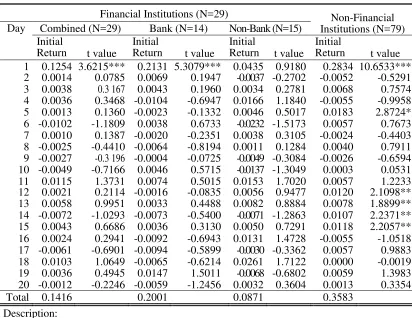
Table 2 shows initial return and significance t level of each group. The values of initial return for financial institutions are less than non-financial institutions during the first 20 trading days in IDX.

(6)

This inconsistent result from previous research on capital markets in Indonesia indicates that there is a significant progress in financial sector supervision so as to reduce the asymmetric information occurs. The less asymmetric information occurs in the financial institutions, the less level of underpricing happened. These results support our expectation on hypothesis 2a.

Table 2. ONE SAMPLE T-TEST ON AVERAGE INITIAL RETURN

Financial Institutions (N=29)

Combined (N=29) Bank (N=14) Non-Bank (N=15)

Non-Financial 1 0.1254 3.6215*** 0.2131 5.3079*** 0.0435 0.9180 0.2834 10.6533*** 2 0.0014 0.0785 0.0069 0.1947 -0.0037 -0.2702 -0.0052 -0.5291 3 0.0038 0.3 167 0.0043 0.1960 0.0034 0.2781 0.0068 0.7574 4 0.0036 0.3468 -0.0104 -0.6947 0.0166 1.1840 -0.0055 -0.9958 5 0.0013 0.1360 -0.0023 -0.1332 0.0046 0.5017 0.0183 2.8724* 6 -0.0102 -1.1809 0.0038 0.6733 -0.0232 -1.5173 0.0057 0.7673 7 0.0010 0.1387 -0.0020 -0.2351 0.0038 0.3105 -0.0024 -0.4403 8 -0.0025 -0.4410 -0.0064 -0.8194 0.0011 0.1284 0.0040 0.7911 9 -0.0027 -0.3 196 -0.0004 -0.0725 -0.0049 -0.3084 -0.0026 -0.6594 10 -0.0049 -0.7166 0.0046 0.5715 -0.0137 -1.3049 0.0003 0.0531 11 0.0115 1.3731 0.0074 0.5015 0.0153 1.7020 0.0057 1.2233 12 0.0021 0.2114 -0.0016 -0.0835 0.0056 0.9477 0.0120 2.1098** 13 0.0058 0.9951 0.0033 0.4488 0.0082 0.8884 0.0078 1.8899** 14 -0.0072 -1.0293 -0.0073 -0.5400 -0.0071 -1.2863 0.0107 2.2371** 15 0.0043 0.6686 0.0036 0.3130 0.0050 0.7291 0.0118 2.2057** 16 0.0024 0.2941 -0.0092 -0.6943 0.0131 1.4728 -0.0055 -1.0518 17 -0.0061 -0.6901 -0.0094 -0.5899 -0.0030 -0.3362 0.0057 0.9883 18 0.0103 1.0649 -0.0065 -0.6214 0.0261 1.7122 0.0000 -0.0019 19 0.0036 0.4945 0.0147 1.5011 -0.0068 -0.6802 0.0059 1.3983 20 -0.0012 -0.2246 -0.0059 -1.2456 0.0032 0.3604 0.0013 0.3354

Total 0.1416 0.2001 0.0871 0.3583

Description:

*significant atα=10% ** significant atα=5% *** significant atα=1%

Sources:Indonesian Stock Exchange and Financial Laboratory Database FBE UBAYA

(7)

Table 3.ONE SAMPLE T-TESTON AVERAGEABNORMAL RETURN

Financial Institutions (N=29)

Combined (N=29) Bank (N=14) Non-Bank (N=15)

Non-Financial

Return t value AbnormalReturn t value AbnormalReturn t value 1 0.1245 3.6332*** 0.2107 5.3605*** 0.0441 0.9301 0.2827 10.6597*** 2 0.0025 0.1366 0.0052 0.1477 -0.0001 -0.0059 -0.0076 -0.7525 3 0.0034 0.2784 0.0098 0.4451 -0.0026 -0.2181 0.0069 0.7783 4 -0.0005 -0.0467 -0.0107 -0.7341 0.0091 0.6675 -0.0068 -1.2547 5 -0.0018 -0.1796 -0.0026 -0.1356 -0.0011 -0.1231 0.0155 2.3954** 6 -0.0090 -0.9568 0.0088 1.2344 -0.0257 -1.5988 0.0076 0.9921 7 -0.0035 -0.4980 -0.0074 -0.8407 0.0001 0.0078 -0.0040 -0.7609 8 0.0003 0.0601 0.0009 0.1276 -0.0002 -0.0269 0.0026 0.5262 9 -0.0007 -0.0786 0.0038 0.5134 -0.0048 -0.3261 -0.0021 -0 .5535 10 -0.0061 -0.8784 0.0042 0.4735 -0.0157 -1.5389 -0.0006 -0.1050 11 0.0049 0.5605 -0.0003 -0.0191 0.0097 1.0436 0.0007 0.1537 12 -0.0028 -0.2651 -0.0063 -0.2996 0.0004 0.0640 0.0095 1.7534* 13 0.0050 0.8525 0.0027 0.3285 0.0072 0.8253 0.0088 2.1648** 14 -0.0041 -0.5468 -0.0033 -0.2260 -0.0048 -0.8383 0.0107 2.2165** 15 0.0073 1.1429 0.0083 0.7980 0.0063 0.7976 0.0109 2.1858** 16 0.0016 0.2238 -0.0117 -1.1153 0.0141 1.5777 -0.0059 -1.1705 17 -0.0038 -0.4439 -0.0094 -0.6232 0.0014 0.1626 0.0079 1.4072 18 0.0077 0.8111 -0.0118 -1.1213 0.0258 1.8215* 0.0015 0.2773 19 0.0017 0.2360 0.0082 0.8560 -0.0043 -0.3878 0.0036 0.8199 20 0.0029 0.4541 -0.0049 -0.9884 0.0101 0.9074 0.0011 0.2721

Total 0.1296 0.1944 0.0691 0.3429

Description:

Sources:Indonesian Stock Exchange and Financial Laboratory Database FBE UBAYA,

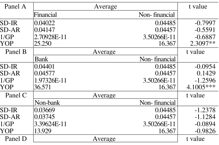
The test of ex-ante uncertainty differences is shown in Table 4. These results show no significant values in all panels. The insignificant results reject hypothesis 3a and 3b. Thus, allegations that have been proposed in hypothesis 3 rejected.

Table 4. EX-ANTE UNCERTAINTY DIFFERENCES TEST

(8)

Non-bank Bank

Table 5 shows the average value of initial return and the level of significance in each comparison group. In the comparison between financial institutions and nonfinancial institutions, t test results showed that the initial returns of the financial institutions are less than non-financial institutions. These results support the t test results in table 2 thus accept the hypothesis 2a. Financial institutions have less asymmetric information than non-financial institutions. This shows that the regulator has managed to reduce the information asymmetry that occurred after the economic crisis in the period 1997-1998. Through tight supervision and better information disclosure, the public can obtain better information about the condition of the financial institutions that have an impact on the less underpricing occurs when enterprises are going public.

Table 5. T TEST DIFFERENCES ON INITIAL RETURN AVERAGES

Population Non- Financial (28,34%) Bank (21,31%)

Financial (12,54%) -3.2449***

-Bank (21,31%) -1.0723***

-Non-Bank (4,35%) -3.7167** -2.7307

Description:

Figures in brackets indicate initial return for each group

Figures in the table shows the statistical t value for the null hypothesis that there is no difference in average initial return for the sample pairs

*significant at a=10% ** significant at a=5% *** significant at a=1%

Another comparison between banks and non-financial institutions results that initial returns of banks are less than non-financial institutions. Comparison between non-bank financial institutions and non-financial institutions also provides the results that initial return of non-bank financial institutions are less than non-financial institutions. These results are consistent with research Alli et al (1994) whose found similar results in their research. Meanwhile, we found insignificant result in comparison between banks and non-banks financial institutions. The results are not significant because of initial return values are not very different.

Table 6. T TEST DIFFERENCES ON ABNORMAL RETURN AVERAGES

Population Non-Financial (28,27%) Bank (21,07%) Financial (12,45%) -3.2615***

Bank (21,07%) -1.1018***

-Non-Bank (4,41%) -3.7071** -2.7069

Description:

Figures in brackets indicate initial return for each group

Figures in the table shows the statistical t value for the null hypothesis that there is no difference in average abnormal return for the sample pairs

*significant at a=10% ** significant at a=5% *** significant at a=1%

(9)

accept hypothesis 2b. These results generally accept hypothesis 2. The other comparisons also provide results that are consistent with the previous table. The results of comparison showed that there was no significant difference between the use of initial returns and abnormal returns to measure the level of significance of the first day return.

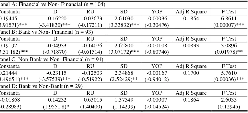
Table 7. REGRESSION TEST ON INITIAL RETURN

Panel A: Financial vs Non- Financial (n = 104)

Constanta D RU SD YOP Adj R Square F Test

0.19445 -0.16220 -0.03673 2.61030 -0.00036 0.1854 6.8611

(3.91571)*** (-3.41830)*** (-0.17211) (3.33832)*** (-0.30476) (0.00007)*** Panel B: Bank vs Non- Financial (n = 93)

0.19197 -0.04933 -0.14076 2.65800 -0.00108 0.0833 3.0896

(3.51 182)*** (-0.71870) (-0.61514) (3.07172)*** (-0.80746) (0.01978)** Panel C: Non-Bank vs Non- Financial (n = 94)

0.21444 -0.23115 -0.12503 2.34868 -0.00167 0.1700 5.7610

(3.4965 1)*** (-3.57539)*** (-0.51922) (2.52429)** (-0.94012) (0.00036)*** Panel D: Bank vs Non-Bank (n = 29)

-0.01868 0.14232 0.63015 1.37549 -0.00007 0.1864 2.6035

(-0.28983) (1.9551 8)* (1.40400) (1.14299) (-0.04524) (0.12945) Description:

IR

I, t= initial return i stock t period

D = dummy variable for different types of firms; with one for the financial institutions and zero for non-financial institutions (A), one for banks and zero for non-financial institutions (B), one for non- bank financial institutions and zero for non-financial sector (C), and one for banks and zero for non- banks financial institutions (D) RU = ratio underwriter reputation ranking

SD = standard deviation of initial returns from the second day the stock traded up to twenty days YOP= number of years from firms was established until first emission of shares

Regression test results in table 7 provide different significances results in each panel. Significant value to the variable types of firms indicates that there is an initial return difference between the financial institutions and non-financial institutions. Negative value coefficient on variable explained that initial returns on financial institutions are smaller than non-financial institutions. These results are consistent with the results of t test on the previous table that the initial return of financial institutions are less than non-financial institutions. This further supports the truth of statement that asymmetric information differences occurred between the financial institutions and nonfinancial institutions as proposed in hypothesis 2. People tend to have more complete information about financial institutions than non-financial institutions.

The other variable that shows significant results is standard deviation. Significant value on the standard deviation of variables explained that the volatility of stock prices affect initial return. The positive coefficient value of standard deviation shows that the larger the standard deviation, the more underpriced the IPO (as measured using the initial return). These results are consistent with the statement that standard deviation has positive effect on underpricing (Ritter, 1984; Alli et al, 1994). These results explain that the standard deviation affect the underpricing of all institutions. Despite of it’s effect on underpricing of IPO, there is no differences in value of standard deviation between financial institutions and non-financial institutions. Thus, the results of regression on the standard deviation of these variables accept hypothesis 4a.

(10)

investors. This conditions force them to make investment decisions without considering reputation of underwriter factor. This insignificant result rejects hypothesis 6a.

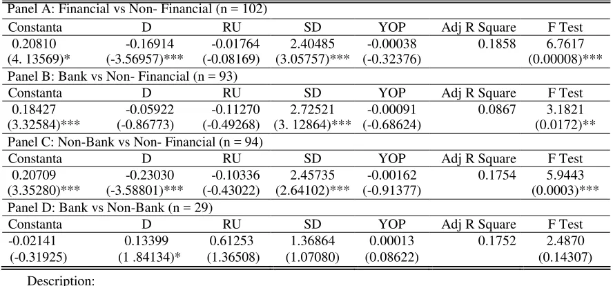
Table 8. REGRESSION TEST ON ABNORMAL RETURN

Panel A: Financial vs Non- Financial (n = 102)

0.20810 -0.16914 -0.01764 2.40485 -0.00038 0.1858 6.7617

(4. 13569)* (-3.56957)*** (-0.08169) (3.05757)*** (-0.32376) (0.00008)*** Panel B: Bank vs Non- Financial (n = 93)

0.18427 -0.05922 -0.11270 2.72521 -0.00091 0.0867 3.1821

(3.32584)*** (-0.86773) (-0.49268) (3. 12864)*** (-0.68624) (0.0172)** Panel C: Non-Bank vs Non- Financial (n = 94)

0.20709 -0.23030 -0.10336 2.45735 -0.00162 0.1754 5.9443

(3.35280)*** (-3.58801)*** (-0.43022) (2.64102)*** (-0.91377) (0.0003)*** Panel D: Bank vs Non-Bank (n = 29)

-0.02141 0.13399 0.61253 1.36864 0.00013 0.1752 2.4870

(-0.31925) (1 .84134)* (1.36508) (1.07080) (0.08622) (0.14307) Description:

ARI, t= abnormal return i stock t period

D = dummy variable for different types of firms; with one for the financial institutions and zero for non-financial institutions (A), one for banks and zero for non-financial institutions (B), one for

non- bank financial institutions and zero for non-financial sector (C), and one for banks and zero for non- banks financial institutions (D) RU = ratio

underwriter reputation ranking

SD = standard deviation of initial returns from the second day the stock traded up to twenty days YOP= number of years from firms was established until first emission of shares

In regression testing with an abnormal return as the dependent variable are presented in Table 8 gives results that are consistent with previous regression testing. Panel A shows significant results on coefficients of variables, types of business entities, and the standard deviation. In the variable types of business entities, the value of the coefficient is negative and significantly explained that the initial return on the financial sector enterprises is smaller than a business enterprise of non-financial sector. These results also support the statement about the information asymmetry differences between the financial sector enterprises and non-financial sector as proposed in hypothesis 2.

Standard deviation positive coefficient values and significant indicates that the standard deviation positively related with abnormal return. These results indicate that both the use of initial return and abnormal return as dependent variables results significant standard deviation values. Standard deviations affect the level of underpricing, but did not show any differences in it’s value between financial institutions and nonfinancial institutions. Based on these results, the hypothesis 4b accepted. With the acceptance of hypotheses 4a and 4b, we accept hypothesis 4.

(11)

The results showed that one, during 2001-2008 period, there was a significant underpricing of IPOs. The financial institutions IPO’s were less underpriced non-financial institutions. This shows that there is asymmetric information difference between the financial institutions and non-financial institutions. Supervision for financial institutions has developed better than the previous few years. Second, there are several factors that affect underpricing significantly. These factors are type of firms and stock trading price volatility in stock exchange.

Third, there is no significant difference in the use of abnormal returns or initial return as a measurement of underpricing of IPO. We found that there is one significance more on abnormal return better than initial return. There is a possibility that the use of market return JCI (km) as a proxy of expected return is less able to give better results than the use of initial return. So that the results in almost all tests showed the similarity in the amount of significance, except on one sample t-test. In this case, both the use of initial return and abnormal return are both good. Fourth, the use of data open to close prices could provide more accurate results for calculation of initial returns and abnormal returns to determine the level of underpricing of IPO.

Based on the results of this study, we recommend investors to consider the types of firms as consideration for investment decision. This is important because investors need to reduce the uncertainty their faces. Investors need to be cautious in investing in stocks that have high underpricing, because there is a greater risk waiting ahead than the stocks with lower underpricing.

Bapepam as expected from the capital market regulators in Indonesia can implement the new rules that could reduce public ignorance about the reputation of the underwriters and firms age. These things can be a public expose more complete on the m e d i a , a l l o w i n g t h e p u b l i c t o h a v e m o r e c o m p l e t e i n f o r m a t i o n . As an important party in the process of initial public offering (IPO), the underwriters need to make a full public exposure in order to give enough information to the public. It is expected that through the full public exposure can reduce the asymmetric information occurs, especially for non-financial institutions. The less asymmetric information occurs, the less level of underpricing occurs too. This will maximize the firms funds need for the purpose of financing its operation activities.

For further research, we recommend continue using the open to close prices in order to get unbiased results in the calculation to measure the level of underpricing. In addition, when using the abnormal return as a measurement, we recommend to use other models other than market adjusted models in order to get more accurate result and prove that this measurement do better to calculate underpricing than initial return. Researchers can also add further factors affecting underpricing such as type of investors.

References

Anadya, Dudi, (2006), “Modul SPSS”, Faculty of Economics University of Surabaya

Allen, F., and G. Faulhaber, 1989, Signalling by Underpricing IPO market, Journal of Financial Economics, Vol.23, pp. 303-323

Alli, K., J. Yau, and K. Yung, 1994, The underpricing of IPOs of Financial Institution, Journal of Business Finance and Accounting, Vol. 21, No.7, (October 1994), pp. 1013- 1039

Brooks, C., 2008, Introductory Econometrics for Finance, Second Edition, Cambridge University Press

Carter, R., and S. Manaster, 1990, Initial Public Offerings and Underwriter Reputation, Journal of Finance, Vol. 45, No. 4, (September 1990), pp. 1045-1067

Ernyan, dan S. Husnan, 1997, “Perbandingan Underpricing Penerbitan Saham Perdana Perusahaan Keuangan dan Non-Keuangan di Pasar Modal Indonesia: Pengujian Hipotesis Asimetri Informasi”, Simposium Nasional Keuangan In Memorian Prof. Dr. Bambang Riyanto

Grinblatt, M., and C. Hwang, 1989, Signalling and the Pricing Of New Issues, Journal of Finance, Vol.44, pp. 393-420

(12)

Jogiyanto, 2008, Teori Portofolio dan Analisis Investasi, Edisi Kelima, BPFE, Yogyakarta

Ibbotson, R.G, 1975, Price Performances of Common Stock New Issues, Journal of Financial Economics, Vol. 2, No. 3, pp. 235-272

Ibbotson, R.G., J.L. Sindelar, and J.R. Ritter, 1987, Initial Public Offerings, Midland Corporate Finance Journal, (Spring 1986), pp. 6-22

Mauer, D.C., and L.C. Senbet, 1992, The Effect of the Secondary Market on the Pricing of Initial Public Offering: Theory and Evidance, Journal of Finance and Quantitative Analysis, Vol. 27, No. 1, pp. 55-79

Michaely, R., and Shaw, W.H., 1994, The Pricing of Initial Public Offerings: Test of Adverse-Selection and Signalling Theories, The review of Financial Studies, Vol. 7, No.2, pp. 279-3 19

Prastisto, A., 2004, Cara Mudah Mengatasi Masalah Statistik Dan Rancangan Percobaan Dengan SPSS 12, Elex Media

Ritter, J., 1984, The Hot Issues Market of 1980, Journal of Business, Vil. 57, pp. 215-241

Rock, K., 1986, Why New Issues Are Underpriced, Journal of Financial Economics, Vol.15, No. 1/2, pp. 187-212

Ross, S. A., R.W. Westerfield, and J. Jaffe, Corporate Finance, Seventh Edition, McGraw Hill International

Ruud, J.S., 1993, “Underwriter Price Support and the IPO Underpricing Puzzle”, Journal of Financial Economics, Vol 34, (March 1993), pp. 135-151

Sulistio, Helen, 2005, “Pengaruh Informasi Akuntansi dan Non Akuntansi Terhadap Initial Return: Studi Pada Perusahaan Yang Melakukan Initial Public Offering Di BEJ”, Simposium Nasional Akuntansi 8, K-AKPM 03, Solo

Sunariyah, 2004, Pengantar Pengetahuan Pasar Modal, Fourth Edition, UPP AMP YKPN, Yogyakarta

Triaryati, N., dan S. Husnan, 2004, “Perbandingan Abnormal Return Emisi Saham Perdana Perusahaan Keuangan dan Non-Keuangan di Pasar Modal Indonesia: Pengujian Terhadap Hipotesis Informasi Asimetri”, Sosiosains, Vol. 17, No.3, (July 2004), pp. 423-441