Closed-form Solutions of Relativistic Black-Scholes
Equations
Yanlin Qu
1,2and Randall R. Rojas
21
School of Mathematical Science
University of Science and Technology of China
2
Department of Economics
University of California, Los Angeles
[email protected], [email protected]
Abstract
Drawing insights from the triumph of relativistic over classical mechanics when ve-locities approach the speed of light, we explore a similar improvement to the seminal Black-Scholes (Black and Scholes (1973)) option pricing formula by considering a rel-ativist version of it, and then finding a respective solution. We show that our solution offers a significant improvement over competing solutions (e.g., Romero and Zubieta-Mart´ınez (2016)), and obtain a new closed-form option pricing formula, containing the speed limit of information transfercas a new parameter. The new formula is rigorously shown to converge to the Black-Scholes formula as cgoes to infinity. Whenc is finite, the new formula can flatten the standard volatility smile which is more consistent with empirical observations. In addition, an alternative family of distributions for stock prices arises from our new formula, which offer a better fit, are shown to converge to lognormal, and help to better explain the volatility skew.
Keywords: Option pricing, Volatility smile, Stock price distribution, Klein-Gordon equation.
1.
Introduction
In agreement with the work done by Romero and Zubieta-Mart´ınez (2016), we take a similar approach for the initial formulation. However, for the purpose of clarity, we simplify the notations by defining
α= 1
where r is the risk-free interest rate, σ is the volatility in the Black-Scholes model, and c
is the speed of light. As usual, let S, K, T be the current stock price, strike price and maturity in the Black-Scholes model respectively. In addition, m represents a mass and~is
the reduced Planck constant. It is well-known that the Black-Scholes equation
∂f
can be mapped to the free Schr¨odinger equation
i~∂ψ
In relativistic quantum mechanics, the free Schr¨odinger equation is replaced by the Klein-Gordon equation
→ψ as c→ ∞(see Schoene and Phillips (1970)). Therefore we apply the inverse map between (1) and (2) with
˜
ψ =e−imc2˜t/~·ψ =eνt·ψ =e−(αx+(β−ν)t)·f
on (3) to obtain the relativistic generalized Black-Scholes equation
In Section 2 we find an explicit solution of (4) which leads to a closed-form option pricing formula, and provide a rigorous proof of convergence as c→ ∞. In Section 3, we show how the new formula and corresponding distribution can flatten the volatility smile/skew from both a theoretical foundation and empirical tests.
2.
The Model
2.1.
Solving the Equation
To illustrate our technique to solve (4) explicitly, we only consider the call option case
with α >0. Other cases can be solved in a similar way. By adding the terminal condition
to (3) and replacing ˜t by it, we instead need to solve
∂2ψ˜ ∂t2 +c
2∂2ψ˜ ∂x2 =ν
2ψ,˜ (x, t)
∈R×(0, T)
˜
ψT =e−(αx+(β−ν)T)(ex−K)+
. (5)
Letϕ(x, t) = ˜ψ(cx, T−t), then the terminal condition becomes the initial condition and we can solve the equation in the upper half plane H =R×R+ instead of R×(0, T). (5) now
can be written as (
∆ϕ=ν2ϕ, (x, t)∈H
ϕ0 =e−(β−ν)T(e(1−α)cx−Ke−αcx)1cx>logK
(6)
where ∆ is the Laplacian and1is the indicator function. Sinceα < 12 by definition,ϕ0grows
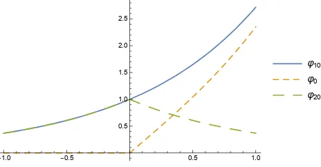
exponentially as x → +∞ so that we can not apply the Fourier Transform to it. Also, it is not smooth at logcK which makes it impossible to obtain an intuitive solution. Therefore, the main insight of our technique is to separate ϕ0 into two parts, a simple part ϕ10 and
an integrable part ϕ20 with ϕ0 = ϕ10 −ϕ20 and ϕ = ϕ1 −ϕ2, where both can be solved
analytically. Figure 1 illustrates our proposed decomposition.
-1.0 -0.5 0.5 1.0
0.5 1.0 1.5 2.0 2.5
φ10
φ0
φ20
For the simple part,
(
∆ϕ1 =ν2ϕ1, (x, t)∈H ϕ10=e−(β−ν)T+(1−α)cx
(7)
we can derive a pair of solutions after several simple observations, namely,
ϕ1 =e−(β−ν)T+(1−α)cx±
is bounded, it is impossible for f0 = f10−f20 to converge to the Black-Scholes formula as c→ ∞. Therefore “−” is the only choice,
f10 =Se(−
√
ν2−(1−α)2c2−(β−ν))T
.
For the integrable part,
(
∆ϕ2 =ν2ϕ2, (x, t)∈H
ϕ20=e−(β−ν)T(e(1−α)cx1cx≤logK+Ke−αcx1cx>logK)
(8)
notice that 0 < α < 1/2 so that ϕ20 has an exponential decay as x → ±∞. Therefore we
can apply a Fourier Transform with respect to x to obtain
where we have used the following two simple formulas (a >0)
Solutions of (9) should be ˆϕ2 = e±
√ ν2+ξ2·t
ˆ
ϕ20. In order to apply the inverse Fourier
Transform on ˆϕ2 to obtain ϕ2, the solutions of (8), ˆϕ2 must be integrable with respect to ξ,
Finally, we get the formula for this case,
f0 =f10−f20=e−βT Se(ν−
For α 6= 0, our technique is valid for both European call and put options. Therefore, after repeating the procedure above, we have
Cc(r, σ, S, T, K) =e−βT Se(ν−
In addition, we have a new put-call parity,
Since (4) → (1) as c → ∞, our new formulas should converge to the Black-Scholes formulas. However, in Section 2.1, we had ruled out several solutions of (4) because they can not converge to the solutions of (1). Therefore, it is possible that our new formulas fail to converge as well. Fortunately, we can eliminate such possibility in this section by providing a rigorous mathematical proof of the convergence. To illustrate the method of the proof explicitly, we only consider the put option case with α < 0. Other cases can be proved in a similar way. Before we start, it is convenient for us to recall the Black-Scholes formulas,
C(r, σ, S, T, K) =SN(d1)−Ke−rTN(d2) (11)
To build a connection between N(·) (the CDF of the normal distribution) in (11) and (12) and the improper integral in (10), we establish the following interesting lemma.
Lemma 2.1. Let θ >0 then
Proof. Denote the integrand above with f(x, τ) (including the constant before the integral) so
finite interval of τ since
By Theorem 11 in Trench (2012), we have
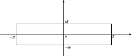
where the last equality holds because of the Fourier Transform from x to τ +θ. Therefore the derivatives of both sides of (14) are always the same so we only need to prove that (14) holds when τ = 0. Consider the complex integral of
h(z) = i 2π
e−z22
z
on the rectangular contour ΓR in the following figure (anticlockwise).
Fig. 2. The rectangular contour ΓR
Notice that h has a simple pole at the origin, by residue theorem,
I
ΓR
h(z)dz = 2πiRes(h,0) = 2πilim
z→0zh(z) =−1.
Since
|h(z)|=
i
2π
e−(x+2iy)2
x+iy
≤
1 2π
e−12R2+ 1 2θ2
R forx=±R and|y| ≤θ,
the integral on two vertical segments vanishes as R → ∞. Notice that the integral on two horizontal segments are the same because h(z) =−h(−z). Let R→ ∞ and finally we have
Z
R
f(x,0)dx=−1 2Rlim→∞
I
ΓR
h(z)dz = 1
2 =N(0).
With the lemma proved, we can prove the convergence now.
Proposition 1. Let α <0 then Pc →P as c→ ∞.
We have
ac-independent function with an exponential decay so that RRf(y, c)dy converges uniformly in [c0,∞). By theorem 10 in Trench (2012) and (15),
σ2T in lemma 2.1, after standard simplification, we
will find that the first term in (16) equals to the first term in (12). Let θ = (1−α)√σ2T,
τ = −d1, x = y
√
σ2T in lemma 2.1, after standard simplification, we will find that the
second term in (16) equals to the second term in (12). Then the proposition is proved.
3.
Distributions And Volatility Smile/Skew
3.1.
Flatten Standard Smiles Directly
After proving the convergence, now we can turn to study the difference between our new formulas and the Black-Scholes formulas. We mainly study formulas for call options here. If we fix r = 0.1, σ = 0.5, S = 50, T = 1, c = 3, then C −Cc is a function of K which
is plotted in the following Figure 3(a). Figure 3(b) shows thatCc is a monotonic increasing
30 40 50 60 70 80
(a) The difference between two formulas
0.3 0.4 0.5 0.6 0.7 0.8
(b) The monotonicity ofCc with respect toσ
Fig. 3. The difference and the monotonicity
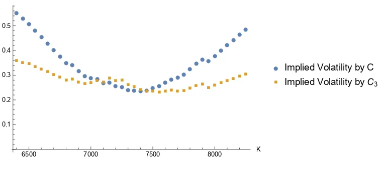
Now we use the data from Appendix B of Fengler (2009) to do an empirical test. It is an implied volatility table of the options on DAX index, June 13, 2000. The DAX spot price on that day is S = 7268.91. In fact, to price options on stock indices or currency options, we need to generalize our new formula by replacing S bySe−qT so that it can deal with options
on stocks paying known dividend yields q. For further discussion of this, see e.g., (Hull and Sankarshan, 2016, p. 402). Fortunately, we do not need to do this here because DAX is a performance index with q= 0. We still choose c= 3 and the result is shown in Figure 4.
●
6500 7000 7500 8000 K
0.1
● Implied Volatility by C
■ Implied Volatility byC3
Fig. 4. Flatten the smile with C3
(Derman and Miller, 2016, p. 149), the smile of those currency options between “equally powerful” currencies (e.g. USD, EUR) can be a standard one. In that case, our new formula may produce a horizontal line.
The choice c= 3 in this subsection is quite arbitrary but it has done a good job. Recall that the real velocity of light is about 3×10⁸. It is an interesting coincidence. Although c is a constant in physics, we need not to fix c = 3 from now on. As we know, light travels at different speed in different mediums. At the same time, different markets have different smiles (Derman and Miller, 2016, p. 131). Therefore, it is reasonable for us to choose different c when we deal with different kinds of options. For example, when we deal with volatility skews of equity options which are more common than smiles, we may need to choose a smaller cin the next subsection.
3.2.
Distributions and Skews
We use the formula from Breeden and Litzenberger (1978) to obtain a new family of distribution for stock price,
gc(K;r, σ, S, T) = erT
∂2C
c
∂K2 =e
(r−β)T 1
2π Sα
K1+α
Z
R
(S/K)iye−(√c2y2+ν2−ν)Tdy (17)
where we do differentiation under the integral sign. We have done the same thing when we prove lemma 2.1. So its validity can be verified in a similar way. Recall the lognormal distribution in the Black-Scholes model with the same parameters,
g(K;r, σ, S, T) = 1
K√2πσ2Te
−(log(K/S2σ)+2Tασ2T)2. (18)
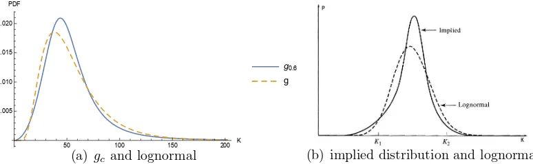
We set c= 0.6 in this subsection and compare (17) with (18) in the following Figure 5(a). Figure 5(b) is from (Hull and Sankarshan, 2016, p. 465) which is used to explain volatility skew of equity options by comparing implied distribution with lognormal distribution.
50 100 150 200 K
0.005 0.010 0.015 0.020 PDF
g0.6
g
(a) gc and lognormal (b) implied distribution and lognormal
To our surprise, when comparing with lognormal, gc in Figure 5(a) has exactly the same
features as the implied distribution in Figure 5(b) such as a heavier left tail near K1, a
sharper peak with deviation to the right, and a less heavy tail near K2. It is interesting to
point out that gc a heavier right tail than lognormal when K is extremely larger than K2.
However, for implied distribution, it is impossible to observe this phenomenon since nobody will trade those options with ridiculously high strike prices. That may be a limitation of option-implied distributions of stock price.
For the convenience of readers, we are going to present the argument in (Hull and Sankar-shan, 2016, p. 465) briefly here to show how Figure 5(b) as well as Figure 5(a) can explain downward volatility skew of equity opitons.
Consider a call with a high strike price K2. Only when the stock price go over K2 can
the option pay off. Such probability is lower for the implied distribution than for lognormal which means the Black-Scholes formula overprices those options. By the monotonicity, the implied volatility is lower than σ in the Black-Scholes model.
Consider a put with a low strike price K1. Only when the stock price drop belowK1 can
the option pay off. Such probability is higher for the implied distribution than for lognormal which means the Black-Scholes formula underprices those options. By the monotonicity, the implied volatility is higher than σ in the Black-Scholes model.
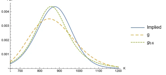
Therefore Figure 5(b) is consistent with downward volatility skew so is Figure 5(a). Then we use the data from (Dar´oczi et al., 2013, p. 97) to do an empirical test. It’s a set of prices of Google call options, June 25, 2013. The price of Google stock on that day is
S = 866.2. We use smooth curves to fit the volatility skew. Using the Black-Scholes formula, we obtain a smooth curve of option prices to which we can apply the formula from Breeden and Litzenberger (1978) again to calculate the implied distribution. In fact, the volatility curve here still looks like a smile but its lowest point is at around 1050 which is much larger than S = 866.2 so we can call it a skew instead. The result is shown in the following figure.
700 800 900 1000 1100 1200K
0.001 0.002 0.003 0.004 PDF
Implied
g
g0.6
It is quite obvious that gc is much closer to the implied distribution than lognormal. Then
we can see the advantage of the new distribution family {gc|c ≥ c0}. It has just one more
parameter cthan lognormal while it has almost all the desired features (see Figure 5) to fit those implied distributions from markets. To the best of the author’s knowledge, there was no distribution family with such properties before. Finally, we prove the following convergence result so that{gc|c≥c0} can be regarded as a powerful generalization of lognormal.
Proposition 2. gc →g as c→ ∞.
Proof. Denote the integrand in (17) withf(y, c) (including the constant before the integral). Repeat the argument in the proof of Proposition 1, then we can take the limit into the integral sign. Then we have
lim
c→∞gc = limc→∞
Z
R
f(y, c)dy=
Z
R lim
c→∞f(y, c)dy
=e−α2σ22T(S/K) α
K·2π
Z
R
e−ilog (K/S)ye−y2σ22Tdy
=e−α2σ22T (S/K) α
K·√2π
1
√
σ2Te
−log (2σK/S2T)2
= 1
K√2πσ2Te
−(log(K/S2σ)+2Tασ2T)2 =g
(19)
where we have used the well-known result (a >0)
[
e−2ta22 =a·e−ω 2a2
2 .
4.
Summary
References
Black, F., Scholes, M., 1973. The pricing of options and corporate liabilities. Journal of political economy 81, 637–654.
Breeden, D. T., Litzenberger, R. H., 1978. Prices of state-contingent claims implicit in option prices. Journal of business pp. 621–651.
Dar´oczi, G., et al., 2013. Introduction to R for Quantitative Finance. Packt Publishing Ltd.
Derman, E., Miller, M. B., 2016. The Volatility Smile. John Wiley & Sons.
Fengler, M. R., 2009. Arbitrage-free smoothing of the implied volatility surface. Quantitative Finance 9, 417–428.
Hull, J. C., Sankarshan, B., 2016. Options, futures, and other derivatives. Pearson Education India, 9th ed.
Romero, J. M., Zubieta-Mart´ınez, I. B., 2016. Relativistic Quantum Finance. ArXiv e-prints .
Schoene, A. Y., Phillips, R., 1970. Semi-groups and a class of singular perturbation problems. Indiana University Mathematics Journal 20, 247–263.