Practical Data Analysis ebook free download

(1)

(2)

Practical Data Analysis

Transform, model, and visualize your data through

hands-on projects, developed in open source tools

Hector Cuesta

(3)

Practical Data Analysis

All rights reserved. No part of this book may be reproduced, stored in a retrieval system, or transmitted in any form or by any means, without the prior written permission of the publisher, except in the case of brief quotations embedded in critical articles or reviews.

Every effort has been made in the preparation of this book to ensure the accuracy of the information presented. However, the information contained in this book is sold without warranty, either express or implied. Neither the author, nor Packt Publishing, and its dealers and distributors will be held liable for any damages caused or alleged to be caused directly or indirectly by this book.

Packt Publishing has endeavored to provide trademark information about all of the companies and products mentioned in this book by the appropriate use of capitals. However, Packt Publishing cannot guarantee the accuracy of this information.

First published: October 2013

Production Reference: 1151013

Published by Packt Publishing Ltd. Livery Place

35 Livery Street

Birmingham B3 2PB, UK. ISBN 978-1-78328-099-5 www.packtpub.com

(4)

(5)

(6)

Foreword

The phrase: From Data to Information, and from Information to Knowledge, has become a cliché but it has never been as fitting as today. With the emergence of Big Data and the need to make sense of the massive amounts of disparate collection of individual datasets, there is a requirement for practitioners of data-driven domains to employ a rich set of analytic methods. Whether during data preparation and cleaning, or data exploration, the use of computational tools has become imperative. However, the complexity of underlying theories represent a challenge for users who wish to apply these methods to exploit the potentially rich contents of available data in their domain. In some domains, text-based data may hold the secret of running a successful business. For others, the analysis of social networks and the classification of sentiments may reveal new strategies for the dissemination of information or the formulation of policy.

(7)

I first met Hector Cuesta during the Fall Semester of 2011, when he joined my Computational Epidemiology Research Laboratory as a visiting scientist. I soon realized that Hector is not just an outstanding programmer, but also a practitioner who can readily apply computational paradigms to problems from different contexts. His expertise in a multitude of computational languages and tools, including Python, CUDA, Hadoop, SQL, and MPI allows him to construct solutions to complex problems from different domains. In this book, Hector Cuesta is demonstrating the application of a variety of data analysis tools on a diverse set of problem domains. Different types of datasets are used to motivate and explore the use of powerful computational methods that are readily applicable to other problem domains. This book serves both as a reference and as tutorial for practitioners to conduct data analysis and move From Data to Information, and from Information to Knowledge.

Armin R. Mikler

Professor of Computer Science and Engineering

(8)

About the Author

Hector Cuesta

holds a B.A in Informatics and M.Sc. in Computer Science. He provides consulting services for software engineering and data analysis with experience in a variety of industries including financial services, social networking, e-learning, and human resources.

He is a lecturer in the Department of Computer Science at the Autonomous

University of Mexico State (UAEM). His main research interests lie in computational epidemiology, machine learning, computer vision, high-performance computing, big data, simulation, and data visualization.

He helped in the technical review of the books, Raspberry Pi Networking Cookbook by Rick Golden and Hadoop Operations and Cluster Management Cookbook by Shumin Guo for Packt Publishing. He is also a columnist at Software Guru magazine and he has published several scientific papers in international journals and conferences. He is an enthusiast of Lego Robotics and Raspberry Pi in his spare time.

(9)

Acknowledgments

I would like to dedicate this book to my wife Yolanda, my wonderful children Damian and Isaac for all the joy they bring into my life, and to my parents Elena and Miguel for their constant support and love.

I would like to thank my great team at Packt Publishing, particular thanks goes to, Anurag Banerjee, Erol Staveley, Edward Gordon, Anugya Khurana, Neeshma Ramakrishnan, Arwa Manasawala, Manal Pednekar, Pragnesh Bilimoria, and Unnati Shah.

Thanks to my friends, Abel Valle, Oscar Manso, Ivan Cervantes, Agustin Ramos, Dr. Rene Cruz, Dr. Adrian Trueba, and Sergio Ruiz for their helpful suggestions and improvements to my drafts. I would also like to thank the technical reviewers for taking the time to send detailed feedback for the drafts.

(10)

About the Reviewers

Mark Kerzner

holds degrees in Law, Math, and Computer Science. He has been designing software for many years, and Hadoop-based systems since 2008. He is the President of SHMsoft, a provider of Hadoop applications for various verticals, and a co-author of the Hadoop Illuminated book/project. He has authored and co-authored books and patents.

I would like to acknowledge the help of my colleagues, in particular Sujee Maniyam, and last but not least I would acknowledge the help of my multi-talented family.

(11)

Ricky J. Sethi

is currently the Director of Research for The Madsci Network and a research scientist at University of Massachusetts Medical Center and UMass Amherst. Dr. Sethi's research tends to be interdisciplinary in nature, relying on machine-learning methods and physics-based models to examine issues in computer vision, social computing, and science learning. He received his B.A. in Molecular and Cellular Biology (Neurobiology)/Physics from the University of California, Berkeley, M.S. in Physics/Business (Information Systems) from the University of Southern California, and Ph.D. in Computer Science (Artificial Intelligence/Computer Vision) from the University of California, Riverside. He has authored or co-authored over 30 peer-reviewed papers or book chapters and was also chosen as an NSF Computing Innovation Fellow at both UCLA and USC's Information Sciences Institute.

Dr. Suchita Tripathi

did her Ph.D. and M.Sc. at Allahabad University in Anthropology. She also has skills in computer applications and SPSS data analysis software. She has language proficiency in Hindi, English, and Japanese. She learned primary and intermediate level Japanese language from ICAS Japanese language training school, Sendai, Japan and received various certificates. She is the author of six articles and one book. She had two years of teaching experience in the Department of Anthropology and Tribal Development, GGV Central University, Bilaspur (C.G.). Her major areas of research are Urban Anthropology, Anthropology of Disasters, Linguistic and Archeological Anthropology.

(12)

(13)

www.PacktPub.com

Support files, eBooks, discount offers and more

You might want to visit www.PacktPub.com for support files and downloads related to your book.

Did you know that Packt offers eBook versions of every book published, with PDF and ePub files available? You can upgrade to the eBook version at www.PacktPub. com and as a print book customer, you are entitled to a discount on the eBook copy. Get in touch with us at service@packtpub.com for more details.

At www.PacktPub.com, you can also read a collection of free technical articles, sign up for a range of free newsletters and receive exclusive discounts and offers on Packt books and eBooks.

TM

http://PacktLib.PacktPub.com

Do you need instant solutions to your IT questions? PacktLib is Packt's online digital book library. Here, you can access, read and search across Packt's entire library of books.

Why Subscribe?

• Fully searchable across every book published by Packt • Copy and paste, print and bookmark content

• On demand and accessible via web browser

Free Access for Packt account holders

(14)

Preface

Practical Data Analysis provides a series of practical projects in order to turn data into insight. It covers a wide range of data analysis tools and algorithms for classification, clustering, visualization, simulation, and forecasting. The goal of this book is to help you understand your data to find patterns, trends, relationships, and insight.

This book contains practical projects that take advantage of the MongoDB, D3.js, and Python language and its ecosystem to present the concepts using code snippets and detailed descriptions.

What this book covers

Chapter 1, Getting Started, discusses the principles of data analysis and the data analysis process.

Chapter 2, Working with Data, explains how to scrub and prepare your data for the analysis and also introduces the use of OpenRefine which is a data cleansing tool.

Chapter 3, Data Visualization, shows how to visualize different kinds of data using D3.js, which is a JavaScript Visualization Framework.

Chapter 4, Text Classification, introduces the binary classification using a Naïve Bayes algorithm to classify spam.

Chapter 5, Similarity-based Image Retrieval, presents a project to find the similarity between images using a dynamic time warping approach.

Chapter 6, Simulation of Stock Prices, explains how to simulate stock prices using Random Walk algorithm, visualized with a D3.js animation.

(23)

Chapter 8, Working with Support Vector Machines, describes how to use support vector machines as a classification method.

Chapter 9, Modeling Infectious Disease with Cellular Automata, introduces the basic concepts of computational epidemiology simulation and explains how to implement a cellular automaton to simulate an epidemic outbreak using D3.js and JavaScript. Chapter 10, Working with Social Graphs, explains how to obtain and visualize your social media graph from Facebook using Gephi.

Chapter 11, Sentiment Analysis of Twitter Data, explains how to use the Twitter API to retrieve data from Twitter. We also see how to improve the text classification to perform a sentiment analysis using the Naïve Bayes algorithm implemented in the Natural Language Toolkit (NLTK).

Chapter 12, Data Processing and Aggregation with MongoDB, introduces the basic operations in MongoDB as well as methods for grouping, filtering, and aggregation.

Chapter 13, Working with MapReduce, illustrates how to use the MapReduce programming model implemented in MongoDB.

Chapter 14, Online Data Analysis with IPython and Wakari, explains how to use the Wakari platform and introduces the basic use of Pandas and PIL with IPython.

Appendix, Setting Up the Infrastructure, provides detailed information on installation of the software tools used in this book.

What you need for this book

The basic requirements for this book are as follows:

• Python • OpenRefine • D3.js • mlpy

• Natural Language Toolkit (NLTK) • Gephi

(24)

Who this book is for

This book is for software developers, analysts, and computer scientists who want to implement data analysis and visualization in a practical way. The book is also intended to provide a self-contained set of practical projects in order to get insight about different kinds of data such as, time series, numerical, multidimensional, social media graphs, and texts. You are not required to have previous knowledge about data analysis, but some basic knowledge about statistics and a general understanding of Python programming is essential.

Conventions

In this book, you will find a number of styles of text that distinguish between different kinds of information. Here are some examples of these styles, and an explanation of their meaning.

Code words in text, database table names, folder names, filenames, file extensions, pathnames, dummy URLs, user input, and Twitter handles are shown as follows: "In this case, we will use the integrate method of the SciPy module to solve the ODE." A block of code is set as follows:

beta = 0.003 gamma = 0.1 sigma = 0.1

def SIRS_model(X, t=0):

r = scipy.array([- beta*X[0]*X[1] + sigma*X[2] , beta*X[0]*X[1] - gamma*X[1]

, gamma*X[1] ] –sigma*X[2]) return r

When we wish to draw your attention to a particular part of a code block, the relevant lines or items are highlighted as follows:

(25)

[ 0 72 153] [ 0 6 219] [ 0 0 225] [ 47 0 178] [153 0 72] [219 0 6] [225 0 0]]

Any command-line input or output is written as follows: db.runCommand( { count: TweetWords })

New terms and important words are shown in bold. Words that you see on the screen, in menus or dialog boxes for example, appear in the text like this: "Next, as we can see in the following screenshot, we will click on the Map Reduce option."

Warnings or important notes appear in a box like this.

Tips and tricks appear like this.

Reader feedback

Feedback from our readers is always welcome. Let us know what you think about this book—what you liked or may have disliked. Reader feedback is important for us to develop titles that you really get the most out of.

To send us general feedback, simply send an e-mail to feedback@packtpub.com, and mention the book title via the subject of your message.

If there is a topic that you have expertise in and you are interested in either writing or contributing to a book, see our author guide on www.packtpub.com/authors.

Customer support

(26)

Downloading the example code

You can download the example code files for all Packt books you have purchased from your account at http://www.packtpub.com. If you purchased this book elsewhere, you can visit http://www.packtpub.com/support and register to have the files e-mailed directly to you.

Errata

Although we have taken every care to ensure the accuracy of our content, mistakes do happen. If you find a mistake in one of our books—maybe a mistake in the text or the code—we would be grateful if you would report this to us. By doing so, you can save other readers from frustration and help us improve subsequent versions of this book. If you find any errata, please report them by visiting http://www.packtpub.com/ submit-errata, selecting your book, clicking on the erratasubmissionform link, and entering the details of your errata. Once your errata are verified, your submission will be accepted and the errata will be uploaded on our website, or added to any list of existing errata, under the Errata section of that title. Any existing errata can be viewed by selecting your title from http://www.packtpub.com/support.

Piracy

Piracy of copyright material on the Internet is an ongoing problem across all media. At Packt, we take the protection of our copyright and licenses very seriously. If you come across any illegal copies of our works, in any form, on the Internet, please provide us with the location address or website name immediately so that we can pursue a remedy.

Please contact us at copyright@packtpub.com with a link to the suspected pirated material.

We appreciate your help in protecting our authors, and our ability to bring you valuable content.

Questions

(27)

(28)

Getting Started

Data analysis is the process in which raw data is ordered and organized, to be used in methods that help to explain the past and predict the future. Data analysis is not about the numbers, it is about making/asking questions, developing explanations, and testing hypotheses. Data Analysis is a multidisciplinary field, which combines Computer Science, Artificial Intelligence & Machine Learning, Statistics & Mathematics, and Knowledge Domain as shown in the following figure:

Computer Science

Knowledge Domain

Statistics & Mathematics Artificial Intelligence & Machine Learning

Data Analysis

Computer science

(29)

Artificial intelligence (AI)

According to Stuart Russell and Peter Norvig:

"[AI] has to do with smart programs, so let's get on and write some."

In other words, AI studies the algorithms that can simulate an intelligent behavior. In data analysis, we use AI to perform those activities that require intelligence such as inference, similarity search, or unsupervised classification.

Machine Learning (ML)

Machine learning is the study of computer algorithms to learn how to react in a certain situation or recognize patterns. According to Arthur Samuel (1959),

"Machine Learning is a field of study that gives computers the ability to learn

without being explicitly programmed."

ML has a large amount of algorithms generally split in to three groups; given how the algorithm is training:

• Supervised learning • Unsupervised learning • Reinforcement learning

Relevant numbers of algorithms are used throughout the book and are combined with practical examples, leading the reader through the process from the data problem to its programming solution.

Statistics

In January 2009, Google's Chief Economist, Hal Varian said,

"I keep saying the sexy job in the next ten years will be statisticians. People think I'm joking, but who would've guessed that computer engineers would've been the sexy job of the 1990s?"

Statistics is the development and application of methods to collect, analyze, and interpret data.

(30)

Mathematics

Data analysis makes use of a lot of mathematical techniques such as linear algebra (vector and matrix, factorization, and eigenvalue), numerical methods, and conditional probability in the algorithms. In this book, all the chapters are self-contained and include the necessary math involved.

Knowledge domain

One of the most important activities in data analysis is asking questions, and a good understanding of the knowledge domain can give you the expertise and intuition needed to ask good questions. Data analysis is used in almost all the domains such as finance, administration, business, social media, government, and science.

Data, information, and knowledge

Data are facts of the world. For example, financial transactions, age, temperature, number of steps from my house to my office, are simply numbers. The information appears when we work with those numbers and we can find value and meaning. The information can help us to make informed decisions.

We can talk about knowledge when the data and the information turn into a set of rules to assist the decisions. In fact, we can't store knowledge because it implies theoretical or practical understanding of a subject. However, using predictive analytics, we can simulate an intelligent behavior and provide a good approximation. An example of how to turn data into knowledge is shown in the following figure:

(31)

The nature of data

Data is the plural of datum, so it is always treated as plural. We can find data in all the situations of the world around us, in all the structured or unstructured, in continuous or discrete conditions, in weather records, stock market logs, in photo albums, music playlists, or in our Twitter accounts. In fact, data can be seen as the essential raw material of any kind of human activity. According to the Oxford English Dictionary:

Data are known facts or things used as basis for inference or reckoning.

As shown in the following figure, we can see Data in two distinct ways: Categorical and Numerical:

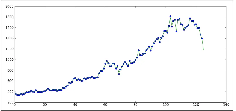
Categorical data are values or observations that can be sorted into groups or categories. There are two types of categorical values, nominal and ordinal. A nominal variable has no intrinsic ordering to its categories. For example, housing is a categorical variable having two categories (own and rent). An ordinal variable has an established ordering. For example, age as a variable with three orderly categories (young, adult, and elder). Numerical data are values or observations that can be measured. There are two kinds of numerical values, discrete and continuous. Discrete data are values or observations that can be counted and are distinct and separate. For example, number of lines in a code. Continuous data are values or observations that may take on any value within a finite or infinite interval. For example, an economic time series such as historic gold prices.

The kinds of datasets used in this book are as follows: • E-mails (unstructured, discrete)

(32)

• Credit approval records (structured, discrete)

• Social media friends and relationships (unstructured, discrete) • Tweets and trending topics (unstructured, continuous)

• Sales records (structured, continuous)

For each of the projects in this book, we try to use a different kind of data. This book is trying to give the reader the ability to address different kinds of data problems.

The data analysis process

When you have a good understanding of a phenomenon, it is possible to make predictions about it. Data analysis helps us to make this possible through exploring the past and creating predictive models.

The data analysis process is composed of the following steps: • The statement of problem

• Obtain your data • Clean the data • Normalize the data • Transform the data • Exploratory statistics • Exploratory visualization • Predictive modeling • Validate your model

• Visualize and interpret your results • Deploy your solution

All these activities can be grouped as shown in the following figure:

(33)

The problem

The problem definition starts with high-level questions such as how to track differences in behavior between groups of customers, or what's going to be the gold price in the next month. Understanding the objectives and requirements from a domain perspective is the key to a successful data analysis project. Types of data analysis questions are listed as follows:

• Inferential • Predictive • Descriptive • Exploratory • Causal • Correlational

Data preparation

Data preparation is about how to obtain, clean, normalize, and transform the data into an optimal dataset, trying to avoid any possible data quality issues such as invalid, ambiguous, out-of-range, or missing values. This process can take a lot of your time. In Chapter 2, Working with Data, we go into more detail about working with data, using OpenRefine to address the complicated tasks. Analyzing data that has not been carefully prepared can lead you to highly misleading results.

The characteristics of good data are listed as follows: • Complete

(34)

Data exploration

Data exploration is essentially looking at the data in a graphical or statistical form trying to find patterns, connections, and relations in the data. Visualization is used to provide overviews in which meaningful patterns may be found.

In Chapter 3, Data Visualization, we present a visualization framework (D3.js) and we implement some examples on how to use visualization as a data exploration tool.

Predictive modeling

Predictive modeling is a process used in data analysis to create or choose a statistical model trying to best predict the probability of an outcome. In this book, we use a variety of those models and we can group them in three categories based on its outcome:

Chapter Algorithm

Categorical outcome (Classification)

4 Naïve Bayes Classifier

11 Natural Language Toolkit + Naïve Bayes Classifier Numerical outcome

(Regression)

6 Random Walk

8 Support Vector Machines 9 Cellular Automata

8 Distance Based Approach + k-nearest neighbor Descriptive modeling

(Clustering)

5 Fast Dynamic Time Warping (FDTW) + Distance

Metrics

10 Force Layout and Fruchterman-Reingold layout

Another important task we need to accomplish in this step is evaluating the model we chose to be optimal for the particular problem.

The No Free Lunch Theorem proposed by Wolpert in 1996 stated:

(35)

The model evaluation helps us to ensure that our analysis is not over-optimistic or over-fitted. In this book, we are going to present two different ways to validate the model:

• Cross-validation: We divide the data into subsets of equal size and test the predictive model in order to estimate how it is going to perform in practice. We will implement cross-validation in order to validate the robustness of our model as well as evaluate multiple models to identify the best model based on their performance.

• Hold-Out: Mostly, large dataset is randomly divided in to three subsets: training set, validation set, and test set.

Visualization of results

This is the final step in our analysis process and we need to answer the following questions:

How is it going to present the results?

For example, in tabular reports, 2D plots, dashboards, or infographics. Where is it going to be deployed?

For example, in hard copy printed, poster, mobile devices, desktop interface, or web. Each choice will depend on the kind of analysis and a particular data. In the

following chapters, we will learn how to use standalone plotting in Python with matplotlib and web visualization with D3.js.

Quantitative versus qualitative data

analysis

Quantitative and qualitative analysis can be defined as follows:

• Quantitative data: It is numerical measurements expressed in terms of numbers

(36)

As shown in the following figure, we can observe the differences between

Quantitative analytics involves analysis of numerical data. The type of the analysis will depend on the level of measurement. There are four kinds of measurements:

• Nominal: Data has no logical order and is used as classification data • Ordinal: Data has a logical order and differences between values are

not constant

• Interval: Data is continuous and depends on logical order. The data has standardized differences between values, but does not include zero • Ratio: Data is continuous with logical order as well as regular interval

differences between values and may include zero

Qualitative analysis can explore the complexity and meaning of social phenomena. Data for qualitative study may include written texts (for example, documents or email) and/or audible and visual data (for example, digital images or sounds). In Chapter 11, Sentiment Analysis of Twitter Data, we present a sentiment analysis from Twitter data as an example of qualitative analysis.

Importance of data visualization

(37)

Many kinds of data visualizations are available such as bar chart, histogram, line chart, pie chart, heat maps, frequency Wordle (as shown in the following figure) and so on, for one variable, two variables, and many variables in one, two, or three dimensions.

Data visualization is an important part of our data analysis process because it is a fast and easy way to do an exploratory data analysis through summarizing their main characteristics with a visual graph.

The goals of exploratory data analysis are listed as follows: • Detection of data errors

• Checking of assumptions

• Finding hidden patterns (such as tendency) • Preliminary selection of appropriate models • Determining relationships between the variables

(38)

What about big data?

Big data is a term used when the data exceeds the processing capacity of typical database. We need a big data analytics when the data grows quickly and we need to uncover hidden patterns, unknown correlations, and other useful information. There are three main features in big data:

• Volume: Large amounts of data

• Variety: Different types of structured, unstructured, and multi-structured data • Velocity: Needs to be analyzed quickly

As shown in the following figure, we can see the interaction between the three Vs:

database, photo, web, video, mobile, social, unstructured

GB TB PB

periodic near real time real time

Variety

Velocity

Volume

(39)

Apache Hadoop is the most popular implementation of MapReduce to solve large-scale distributed data storage, analysis, and retrieval tasks. However,

MapReduce is just one of the three classes of technologies for storing and managing big data. The other two classes are NoSQL and massively parallel processing (MPP) data stores. In this book, we implement MapReduce functions and NoSQL storage through MongoDB, see Chapter 12, Data Processing and Aggregation with MongoDB and Chapter 13, Working with MapReduce.

MongoDB provides us with document-oriented storage, high availability, and map/reduce flexible aggregation for data processing.

A paper published by the IEEE in 2009, The Unreasonable Effectiveness of Data states: But invariably, simple models and a lot of data trump over more elaborate models based on less data.

This is a fundamental idea in big data (you can find the full paper at http://bit. ly/1dvHCom). The trouble with real world data is that the probability of finding false correlations is high and gets higher as the datasets grow. That's why, in this book, we focus on meaningful data instead of big data.

One of the main challenges for big data is how to store, protect, backup, organize, and catalog the data in a petabyte scale. Another main challenge of big data is the concept of data ubiquity. With the proliferation of smart devices with several sensors and cameras the amount of data available for each person increases every minute. Big data must process all this data in real time.

Better

Algorithms Vs. More Data Vs. Better Data

Sensors and cameras

Interaction with the outside world is highly important in data analysis. Using sensors such as RFID (Radio-frequency identification) or a smartphone to scan a QR code (Quick Response Code) is an easy way to interact directly with the customer, make recommendations, and analyze consumer trends.

(40)

The interaction with the real world can give you a competitive advantage and a real-time data source directly from the customer.

Social networks analysis

(41)

Social networks are strongly connected and these connections are often not symmetric. This makes the SNA computationally expensive, and needs to be addressed with high-performance solutions that are less statistical and more algorithmic.

The visualization of a social network can help us to get a good insight into how people are connected. The exploration of the graph is done through displaying nodes and ties in various colors, sizes, and distributions. The D3.js library has animation capabilities that enable us to visualize the social graph with an interactive animation. These help us to simulate behaviors such as information diffusion or distance

between nodes.

Facebook processes more than 500 TB data daily (images, text, video, likes, and relationships), this amount of data needs non-conventional treatment such as NoSQL databases and MapReduce frameworks, in this book, we work with MongoDB—a document-based NoSQL database, which also has great functions for aggregations and MapReduce processing.

Tools and toys for this book

The main goal of this book is to provide the reader with self-contained projects ready to deploy, in order to do this, as you go through the book you will use and implement tools such as Python, D3, and MongoDB. These tools will help you to program and deploy the projects. You also can download all the code from the author's GitHub repository https://github.com/hmcuesta.

You can see a detailed installation and setup process of all the tools in Appendix, Setting Up the Infrastructure.

Why Python?

Python is a scripting language—an interpreted language with its own built-in memory management and good facilities for calling and cooperating with other programs. There are two popular Versions, 2.7 or 3.x, in this book, we will focused on the 3.x Version because it is under active development and has already seen over two years of stable releases.

(42)

Python is excellent for beginners, yet great for experts and is highly scalable— suitable for large projects as well as small ones. Also it is easily extensible and object-oriented.

Python is widely used by organizations such as Google, Yahoo Maps, NASA, RedHat, Raspberry Pi, IBM, and so on.

A list of organizations using Python is available at http://wiki.python.org/moin/ OrganizationsUsingPython.

Python has excellent documentation and examples at http://docs.python.org/3/. Python is free to use, even for commercial products, download is available for free from http://python.org/.

Why mlpy?

mlpy (Machine Learning Python) is a Python module built on top of NumPy, SciPy, and the GNU Scientific Libraries. It is open source and supports Python 3.x. The mlpy module has a large amount of machine learning algorithms for supervised and unsupervised problems.

Some of the features of mlpy that will be used in this book are as follows:

• We will perform a numeric regression with kernel ridge regression (KRR) • We will explore the dimensionality reduction through principal component

analysis (PCA)

• We will work with support vector machines (SVM) for classification • We will perform text classification with Naive Bayes

• We will see how different two time series are with dynamic time warping (DTW) distance metric

We can download the latest Version of mlpy from http://mlpy.sourceforge.net/. For reference you can refer to the paper mply: Machine Learning Python

(43)

Why D3.js?

D3.js (Data-Driven Documents) was developed by Mike Bostock. D3 is a JavaScript library for visualizing data and manipulating the document object model that runs in a browser without a plugin. In D3.js you can manipulate all the elements of the DOM (Document Object Model); it is as flexible as the client-side web technology stack (HTML, CSS, and SVG).

D3.js supports large datasets and includes animation capabilities that make it a really good choice for web visualization.

D3 has an excellent documentation, examples, and community at https://github. com/mbostock/d3/wiki/Gallery and https://github.com/mbostock/d3/wiki. You can download the latest Version of D3.js from http://d3js.org/d3.v3.zip.

Why MongoDB?

NoSQL (Not only SQL) is a term that covers different types of data storage

technologies, used when you can't fit your business model into a classical relational data model. NoSQL is mainly used in Web 2.0 and in social media applications.

MongoDB is a document-based database. This means that MongoDB stores and organizes the data as a collection of documents that gives you the possibility to store the view models almost exactly like you model them in the application. Also, you can perform complex searches for data and elementary data mining with MapReduce. MongoDB is highly scalable, robust, and perfect to work with JavaScript-based web applications because you can store your data in a JSON (JavaScript Object Notation) document and implement a flexible schema which makes it perfect for no structured data.

MongoDB is used by highly recognized corporations such as Foursquare, Craigslist, Firebase, SAP, and Forbes. We can see a detailed list at http://www.mongodb.org/ about/production-deployments/.

MongoDB has a big and active community and well-written documentation at http://docs.mongodb.org/manual/.

(44)

Summary

In this chapter, we presented an overview of the data analysis ecosystem, explaining basic concepts of the data analysis process, tools, and some insight into the practical applications of the data analysis. We have also provided an overview of the different kinds of data; numerical and categorical. We got into the nature of data, structured (databases, logs, and reports) and unstructured (image collections, social networks, and text mining). Then, we introduced the importance of data visualization and how a fine visualization can help us in the exploratory data analysis. Finally we explored some of the concepts of big data and social networks analysis.

In the next chapter, we will work with data, cleaning, processing, and transforming, using Python and OpenRefine.

Downloading the example code

You can download the example code files for all Packt books you

have purchased from your account at http://www.packtpub.com. If you purchased this book elsewhere, you can visit http://www. packtpub.com/support and register to have the files e-mailed

(45)

(46)

Working with Data

Building real world's data analytics requires accurate data. In this chapter we discuss how to obtain, clean, normalize, and transform raw data into a standard format such as Comma-Separated Values (CSV) or JavaScript Object Notation (JSON) using OpenRefine.

In this chapter we will cover: • Datasource

° Open data ° Text files ° Excel files ° SQL databases ° NoSQL databases ° Multimedia ° Web scraping

• Data scrubbing

° Statistical methods ° Text parsing

° Data transformation • Data formats

° CSV

° JSON

° XML

° YAML

(47)

Datasource

Datasource is a term used for all the technology related to the extraction and storage of data. A datasource can be anything from a simple text file to a big database. The raw data can come from observation logs, sensors, transactions, or user's behavior. In this section we will take a look into the most common forms for datasource and datasets.

A dataset is a collection of data, usually presented in tabular form. Each column represents a particular variable, and each row corresponds to a given member of the data, as is shown in the following figure:

A dataset represents a physical implementation of a datasource; the common features of a dataset are as follows:

• Dataset characteristics (such as multivariate or univariate) • Number of instances

• Area (for example life, business, and so on)

(48)

• Number of attributes

• Associated tasks (such as classification or clustering) • Missing Values

Open data

Open data is data that can be used, re-use, and redistributed freely by anyone for any purpose. Following is a short list of repositories and databases for open data:

• Datahub is available at http://datahub.io/

• Book-Crossing Dataset is available at http://www.informatik.uni-freiburg.de/~cziegler/BX/

• World Health Organization is available at http://www.who.int/research/en/

• The World Bank is available at http://data.worldbank.org/ • NASA is available at http://data.nasa.gov/

• United States Government is available at http://www.data.gov/ • Machine Learning Datasets is available at

http://bitly.com/bundles/bigmlcom/2

• Scientific Data from University of Muenster is available at http://data.uni-muenster.de/

• Hilary Mason research-quality datasets is available at https://bitly.com/bundles/hmason/1

Other interesting sources of data come from the data mining and knowledge discovery competitions such as ACM-KDD Cup or Kaggle platform, in most cases the datasets are still available, even after the competition is closed.

Check out the ACM-KDD Cup at the link http://www.sigkdd. org/kddcup/index.php.

(49)

Text files

The text files are commonly used for storage of data, because it is easy to transform into different formats, and it is often easier to recover and continue processing the remaining contents than with other formats. Large amounts of data come in text format from logs, sensors, e-mails, and transactions. There are several formats for text files such as CSV (comma delimited), TSV (tab delimited), Extensible Markup Language (XML) and (JSON) (see the Data formats section).

Excel files

MS-Excel is probably the most used and also the most underrated data analysis tool. In fact Excel has some good points such as filtering, aggregation functions, and using Visual Basis for Application you can make Structured Query Language (SQL)—such as queries with the sheets or with an external database.

Excel provides us with some visualization tools and we can extend the analysis capabilities of Excel (Version 2010) by installing the Analysis ToolPak that includes functions for Regression, Correlation, Covariance, Fourier Analysis, and so on. For more information about the Analysis ToolPak check the link http://bit.ly/ZQKwSa. Some Excel disadvantages are that missing values are handled inconsistently and there is no record of how an analysis was accomplished. In the case of the Analysis ToolPak, it can only work with one sheet at a time. That's why Excel is a poor choice for statistical analysis beyond the basic examples.

(50)

SQL databases

A database is an organized collection of data. SQL is a database language for managing and manipulating data in Relational Database Management Systems (RDBMS). The Database Management Systems (DBMS) are responsible for

maintaining the integrity and security of stored data, and for recovering information if the system fails. SQL Language is split into two subsets of instructions, the Data Definition Language (DDL) and Data Manipulation Language (DML).

The data is organized in schemas (database) and divided into tables related by logical relationships, where we can retrieve the data by making queries to the main schema, as is shown in the following screenshot:

DDL allows us to create, delete, and alter database tables. We can also define keys to specify relationships between tables, and implement constraints between database tables.

• CREATE TABLE: This command creates a new table • ALTER TABLE: This command alters a table

• DROP TABLE: This command deletes a table

DML is a language which enables users to access and manipulate data. • SELECT: This command retrieves data from the database

• INSERT INTO: This command inserts new data into the database • UPDATE: This command modifies data in the database

(51)

NoSQL databases

Not only SQL (NoSQL) is a term used in several technologies where the nature of the data does not require a relational model. NoSQL technologies allow working with a huge quantity of data, higher availability, scalability, and performance.

See Chapter 12, Data Processing and Aggregation with MongoDB and Chapter 13, Working with MapReduce, for extended examples of document store database MongoDB. The most common types of NoSQL data stores are:

• Document store: Data is stored and organized as a collection of documents. The model schema is flexible and each collection can handle any number of fields. For example, MongoDB uses a document of type BSON (binary format of JSON) and CouchDB uses a JSON document.

• Key-value store: Data is stored as key-value pairs without a predefined schema. Values are retrieved from their keys. For example, Apache Cassandra, Dynamo, HBase, and Amazon SimpleDB.

• Graph-based store: Data is stored in graph structures with nodes, edges, and properties using the computer science graph theory for storing and retrieving data. These kinds of databases are excellent to represent social network relationships. For example, Neo4js, InfoGrid, and Horton.

For more information about NoSQL see the following link: http://nosql-database.org/

Multimedia

The increasing number of mobile devices makes it a priority of data analysis to acquire the ability to extract semantic information from multimedia datasources. Datasources include directly perceivable media such as audio, image, and video. Some of the applications for these kinds of datasources are as follows:

• Content-based image retrieval • Content-based video retrieval • Movie and video classification • Face recognition

• Speech recognition

• Audio and music classification

(52)

Web scraping

When we want to obtain data, a good place to start is in the web. Web scraping refers to an application that processes the HTML of a web page to extract data for manipulation. Web scraping applications will simulate a person viewing a website with a browser. In the following example, we assume we want to get the current gold price from the website www.gold.org, as is shown in the following screenshot:

Then we need to inspect the Gold Spot Price element in the website, where we will find the following HTML tag:

We can observe an id, spotpriceCellAsk in the td tag; this is the element we will get with the next Python code.

For this example, we will use the library BeautifulSoup Version 4, in

Linux we can install it from the system package manager, we need to open a Terminal and execute the next command:

$ apt-get install python-bs4

For windows we need to download the library from the following link:

http://crummy.com/software/BeautifulSoup/bs4/download/

To install it, just execute in the command line:

$ python setup.py install

1. First we need to import the libraries BeautifulSoup and urllib.request from bs4 import BeautifulSoup

import urllib.request from time import sleep

(53)

2. Then we use the function getGoldPrice to retrieve the current price from the website, in order to do this we need to provide the URL to make the request and read the entire page.

req = urllib.request.urlopen(url) page = req.read()

3. Next, we use BeautifulSoup to parse the page (creating a list of all the elements of the page) and ask for the element td with the id, spotpriceCellAsk:

scraping = BeautifulSoup(page)

price= scraping.findAll("td",attrs={"id":"spotpriceCellAsk"})[0]. text

4. Now we return the variable price with the current gold price, this value changes every minute on the website, in this case, we want all the values in an hour, so we call the function getGoldPrice in a for loop 60 times, making the script wait 59 seconds between each call.

for x in range(0,60): ...

sleep(59)

5. Finally, we save the result in a file goldPrice.out and include the current date time in the format HH:MM:SS (A.M. or P.M.), for example, 11:35:42PM, separated by a comma.

with open("goldPrice.out","w") as f: ...

sNow = datetime.now().strftime("%I:%M:%S%p")

f.write("{0}, {1} \n ".format(sNow, getGoldPrice()))

The function datetime.now().strftime creates a string representing the time under the control of an explicit format string "%I:%M:%S%p", where %I represents hour as decimal number from 0 to 12, %M represents minute as a decimal number from 00 to 59, %S represents second as a decimal number from 00 to 61, and %p represent either A.M. or P.M.

(54)

The following is the full script: from bs4 import BeautifulSoup import urllib.request

from time import sleep

from datetime import datetime def getGoldPrice():

url = "http://gold.org"

req = urllib.request.urlopen(url) page = req.read()

scraping = BeautifulSoup(page)

price= scraping.findAll("td",attrs={"id":"spotpriceCellAsk"})[0] .text

return price

with open("goldPrice.out","w") as f: for x in range(0,60):

sNow = datetime.now().strftime("%I:%M:%S%p")

f.write("{0}, {1} \n ".format(sNow, getGoldPrice())) sleep(59)

You can download the full script (WebScraping.py) from the author's GitHub repository, which is available at https:// github.com/hmcuesta/PDA_Book/tree/master/Chapter2

The output file, goldPrice.out, will look as follows: 11:35:02AM, 1481.25

(55)

Data scrubbing

Data scrubbing, also called data cleansing, is the process of correcting or removing data in a dataset that is incorrect, inaccurate, incomplete, improperly formatted, or duplicated.

The result of the data analysis process not only depends on the algorithms, it also depends on the quality of the data. That's why the next step after obtaining the data, is data scrubbing. In order to avoid dirty data our dataset should possess the following characteristics:

The dirty data can be detected by applying some simple statistical data validation also by parsing the texts or deleting duplicate values. Missing or sparse data can lead you to highly misleading results.

Statistical methods

In this method we need some context about the problem (knowledge domain) to find values that are unexpected and thus erroneous, even if the data type match but the values are out of the range, it can be resolved by setting the values to an average or mean value. Statistical validations can be used to handle missing values which can be replaced by one or more probable values using Interpolation or by reducing the dataset using Decimation.

• Mean: This is the value calculated by summing up all values and then dividing by the number of values.

• Median: The median is the middle value in a sorted list of values.

• Range Constraints: The numbers or dates should fall within a certain range. That is, they have minimum and/or maximum possible values.

(56)

Text parsing

We perform parsing to help us to validate if a string of data is well formatted and avoid syntax errors.

Regular expression patterns, usually text fields, would have to be validated in this way. For example, dates, e-mails, phone numbers, and IP addresses. Regex is a common abbreviation for regular expression.

In Python we will use the re module to implement regular expressions. We can perform text search and pattern validations.

Firstly, we need to import the re module. import re

In the following examples, we will implement three of the most common validations (e-mail, IP address, and date format):

• E-mail validation:

myString = 'From: readers@packt.com (readers email)' result = re.search('([\w.-]+)@([\w.-]+)', myString)

The function search() scans through a string, searching for any location where the regex might match. The function group() helps us to return the string matched by the regex. The pattern \w matches any alphanumeric character and is equivalent to the class (a-z, A-Z, 0-9_).

• IP address validation:

isIP = re.compile('\d{1,3}\.\d{1,3}\.\d{1,3}\.\d{1,3}') myString = " Your IP is: 192.168.1.254 "

result = re.findall(isIP,myString) print(result)

Output:

(57)

The function findall() finds all the substrings where the regex matches, and returns them as a list. The pattern \d matches any decimal digit, is equivalent to the class [0-9].

• Date format:

print("invalid") Output:

>>> 'valid'

The function match() finds if the regex matches with the string. The pattern implements the class [0-9] in order to parse the date format.

For more information about regular expressions, visit the link

http://docs.python.org/3.2/howto/regex.html#regex-howto.

Data transformation

Data transformation is usually related to databases and data warehouses, where values from a source format are extracted, transformed, and loaded in a destination format.

Extract, Transform, and Load (ETL) obtains data from datasources, performs some transformation function depending on our data model and loads the result data into destination.

• Data extraction allows us to obtain data from multiple datasources, such as relational databases, data streaming, text files (JSON, CSV, XML), and NoSQL databases.

(58)

• Data loading allows us to load data into destination format, such as relational databases, text files (JSON, CSV, XML), and NoSQL databases.

In statistics, data transformation refers to the application of a mathematical function to the dataset or time series points.

Data formats

When we are working with data for human consumption the easiest way to store it is through text files. In this section, we will present parsing examples of the most common formats such as CSV, JSON, and XML. These examples will be very helpful in the next chapters.

The dataset used for these examples is a list of Pokémon characters by National Pokedex number, obtained at the URL http://bulbapedia. bulbagarden.net/.

All the scripts and dataset files can be found in the author's GitHub

repository available at the URL https://github.com/hmcuesta/ PDA_Book/tree/master/Chapter3/.

CSV

(59)

There are many ways to parse a CSV file from Python, and in a moment we will discuss two of them:

The first eight records of the CSV file (pokemon.csv) look as follows: id, typeTwo, name, type

001, Poison, Bulbasaur, Grass 002, Poison, Ivysaur, Grass 003, Poison, Venusaur, Grass 006, Flying, Charizard, Fire 012, Flying, Butterfree, Bug 013, Poison, Weedle, Bug 014, Poison, Kakuna, Bug 015, Poison, Beedrill, Bug . . .

Parsing a CSV file with the csv module

Firstly, we need to import the csv module: import csv

Then we open the file .csv and with the function csv.reader(f) we parse the file: with open("pokemon.csv") as f:

(60)

Parsing a CSV file using NumPy

Perform the following steps for parsing a CSV file:

1. Firstly, we need to import the numpy library: import numpy as np

2. NumPy provides us with the genfromtxt function, which receives four parameters. First, we need to provide the name of the file pokemon.csv. Then we skip first line as a header (skip_header). Next we need to specify the data type (dtype). Finally, we will define the comma as the delimiter. data = np.genfromtxt("pokemon.csv"

,skip_header=1 ,dtype=None ,delimiter=',')

3. Then just print the result. print(data)

Output:

id: id , typeTwo: typeTwo, name: name, type: type

id: 001 , typeTwo: Poison, name: Bulbasaur, type: Grass

JSON is a common format to exchange data. Although it is derived from JavaScript, Python provides us with a library to parse JSON.

Parsing a JSON file using json module

(61)

"id": " 002",

Firstly, we need to import the json module and pprint (pretty-print) module. import json

from pprint import pprint

Then we open the file pokemon.json and with the function json.loads we parse the file.

with open("pokemon.json") as f: data = json.loads(f.read())

(62)

XML

According with to World Wide Web Consortium (W3C) available at http://www.w3.org/XML/

Extensible Markup Language (XML) is a simple, very flexible text format derived

from SGML (ISO 8879). Originally designed to meet the challenges of large-scale electronic publishing, XML is also playing an increasingly important role in the exchange of a wide variety of data on the Web and elsewhere.

The first three records of the XML file (pokemon.xml) look as follows: <?xml version="1.0" encoding="UTF-8" ?>

<typeTwo> Poison</typeTwo> <name> Bulbasaur</name> <type> Grass</type> </row>

<row>

<typeTwo> Poison</typeTwo> <name> Ivysaur</name> <type> Grass</type> </row>

<row>

<typeTwo> Poison</typeTwo> <name> Venusaur</name> <type> Grass</type> </row>

. . . </pokemon>

Parsing an XML file in Python using xml module

Firstly, we need to import the ElementTree object from xml module. from xml.etree import ElementTree

Then we open the file "pokemon.xml" and with the function ElementTree.parse we parse the file.

(63)

Finally, just print each 'row' element with the findall function: for node in doc.findall('row'):

print("")

print("id: {0}".format(node.find('id').text))

print("typeTwo: {0}".format(node.find('typeTwo').text)) print("name: {0}".format(node.find('name').text)) print("type: {0}".format(node.find('type').text))

YAML Ain't Markup Language (YAML) is a human-friendly data serialization format. It's not as popular as JSON or XML but it was designed to be easily mapped to data types common to most high-level languages. A Python parser implementation called PyYAML is available in PyPI repository and its implementation is very similar to the JSON module.

(64)

name : Ivysaur type : Grass -id : 003 typeTwo : Poison name : Venusaur type : Grass . . .

Getting started with OpenRefine

OpenRefine (formerly known as Google Refine) is a formatting tool very useful in data cleansing, data exploration, and data transformation. It is an open source web application which runs directly in your computer, skipping the problem of uploading your delicate information to an external server.

To start working with OpenRefine just run the application and open a browser in the URL available at http://127.0.0.1:3333/.

Refer to Appendix, Setting Up the Infrastructure.

Firstly, we need to upload our data and click on Create Project. In the following screenshot, we can observe our dataset, in this case, we will use monthly sales of an alcoholic beverages company. The dataset format is an MS Excel (.xlsx) worksheet with 160 rows.

We can download the original MS Excel file and the OpenRefine project from the author's GitHub repository available at the following URL:

(65)

Text facet

Text facet is a very useful tool, similar to filter in a spreadsheet. Text facet groups unique text values into groups. This can help us to merge information and we can see values, which could be spelled in a lot of different ways.

Now we will create a text facet on the name column by clicking on that column's drop-down menu and select Facet|Text Facet. In the following screenshot we can see the column name grouped by its content. This is helpful to see the distribution of elements in the dataset. We will observe the number of choices (43 in this example) and we can sort the information by name or by count.

Clustering

(66)

Practical Data Analysis ebook free download

Practical Data Analysis

Transform, model, and visualize your data through

hands-on projects, developed in open source tools

Hector Cuesta

Practical Data Analysis

Foreword

About the Author

Hector Cuesta

Acknowledgments

About the Reviewers

Mark Kerzner

Ricky J. Sethi

Dr. Suchita Tripathi

www.PacktPub.com

Support files, eBooks, discount offers and more

Why Subscribe?

Free Access for Packt account holders

Table of Contents

Preface 1

Chapter 1: Getting Started

7

Chapter 2: Working with Data

25

Chapter 3: Data Visualization

51

Chapter 4: Text Classification

79

Chapter 5: Similarity-based Image Retrieval

93

Chapter 6: Simulation of Stock Prices

105

Chapter 7: Predicting Gold Prices

119

Chapter 8: Working with Support Vector Machines

135

Chapter 9: Modeling Infectious Disease with Cellular Automata 153

Chapter 10: Working with Social Graphs

175

Chapter 11: Sentiment Analysis of Twitter Data

199

Chapter 12: Data Processing and Aggregation with MongoDB

225

Chapter 13: Working with MapReduce

247

Chapter 14: Online Data Analysis with IPython and Wakari

269

Appendix: Setting Up the Infrastructure

301

Preface

What this book covers

What you need for this book

Who this book is for

Conventions

Reader feedback

Customer support

Downloading the example code

Errata

Piracy

Questions

Getting Started

Computer science

Artificial intelligence (AI)

Machine Learning (ML)

Statistics

Mathematics

Knowledge domain

Data, information, and knowledge

The nature of data

The data analysis process

The problem

Data preparation

Data exploration

Predictive modeling

Visualization of results

Quantitative versus qualitative data

analysis

Importance of data visualization

What about big data?

Sensors and cameras