A GEOGRAPHIC WEIGHTED REGRESSION FOR RURAL HIGHWAYS CRASHES
MODELLING USING THE GAUSSIAN AND TRICUBE KERNELS: A CASE STUDY OF
USA RURAL HIGHWAYS
Mohammad Aghayari a, Parham Pahlavani a,*, Behnaz Bigdeli b
a School of Surveying and Geospatial Engineering, College of Engineering, University of Tehran, Tehran, Iran b School of Civil Engineering, Shahrood University of Technology, Shahrood, Iran.
(aghayari.mohammad, [email protected]; [email protected])
KEY WORDS: Geographic Weighted Regression, Ordinary Least Squares, Rural highways crashes modelling, USA Highways, Spatial autocorrelation, Spatial non-stationarity
ABSTRACT:
Based on world health organization (WHO) report, driving incidents are counted as one of the eight initial reasons for death in the world. The purpose of this paper is to develop a method for regression on effective parameters of highway crashes. In the traditional methods, it was assumed that the data are completely independent and environment is homogenous while the crashes are spatial events which are occurring in geographic space and crashes have spatial data. Spatial data have spatial features such as spatial autocorrelation and spatial non-stationarity in a way working with them is going to be a bit difficult. The proposed method has implemented on a set of records of fatal crashes that have been occurred in highways connecting eight east states of US. This data have been recorded between the years 2007 and 2009. In this study, we have used GWR method with two Gaussian and Tricube kernels. The Number of casualties has been considered as dependent variable and number of persons in crash, road alignment, number of lanes, pavement type, surface condition, road fence, light condition, vehicle type, weather, drunk driver, speed limitation, harmful event, road profile, and junction type have been considered as explanatory variables according to previous studies in using GWR method. We have compered the results of implementation with OLS method. Results showed that R2 for OLS method is 0.0654 and for the proposed method is 0.9196 that implies the proposed GWR is better method for regression in rural highway crashes.
1. INTRODUCTION
Driving incidents and their social and economical impacts have compelled UN that call current decade as the decade for the secure roads. Based on world health organization (WHO) report, driving incidents are counted as one of eight reasons for death in the world (PARK et al., 2010).
Among the various components of country’s infrastructure, the roads are very important in the transport of goods and passengers. Therefore, road safety authorities around the world demanding for use of new technologies in vehicles an infrastructure to enhance roads safety.
Basically, crashes are spatial events which occur in geographic space. Traffic crashes can be spatially the correlated events and the analysis of the distribution of traffic crash frequency requires the evaluation of parameters that reflects the spatial properties and correlation (Rhee et al., 2016). Most of accidents occur due to human faults, technical failure of vehicle, technical failure of road, and environmental condition. Sometimes, accumulation of these factors as the hidden factors lead to accident.
Accumulation of several factors create the hotspots. Identifying effective parameters of accidents can prevent future incidents (Black, 1991).
Previous studies have used regression analysis to determine effective parameters. Crashes severity models like linear least square, negative binomial regression, Poisson and more complex models like seemingly unrelated regression have been most former common methods.
Chen et al (2016) developed a hierarchical Bayesian logistic model to examine the significant factors at crash and vehicle/driver levels and their heterogeneous impact on driver
injury in rural interstate highway crashes. Rhee et al (2016) have employed a geographic weighted regression in urban traffic analysis in Seoul. The result showed the best area for safety improvement and because center lanes had more crashes, there is a need to improve the design to enhance their safety. De Oña et al (2013) have used the combination of Latent Class Clustering (LCC) and Bayesian networks (BN). The result showed that the simultaneous use of these methods is useful for road safety analysis. Xu and Huang (2015) have employed the semi-parametric geographically weighted Poisson regression model (S-GWPR) and the random parameter negative binomial model (RPNB) to investigate the spatial heterogeneity in regional crash modelling. The result showed that the S-GWPR is more appropriate for regional crash modelling in comparison with those of the non-spatial models and global models. Zha et al (2016) have used Poisson inverse Gussian (PIG) regression model for modelling motor vehicle crash data and compered it with Negative binomial (NB) model. The result showed the PIG models perform better than the NB in the term of goodness of fit statistics and the PIG model can perform as well as NB model in capturing the variance of crash data. Also PIG models demonstrate same prediction performance compared to NB models. Hence, PIG model could be alternative to NB model for analysing the crash data.
driver failure. In 70.5%, crashes caused by the environment and in 31.5%, technical failure of vehicles was the reason of the incidents.
(Kashani and Mohaymany, 2011) used a classification and regression tree (CART) to determine both the severity of crashes and the effective factors on the severity of injury for passengers on two lane two way roads.
As mentioned above, lots of studies have been conducted to find appropriate methods for detecting effective factors in crashes but most of this studies have not considered spatial data’s features properly.
Basic regression models assumes that data should be independent but this assumption is impossible in spatial data. Spatial data have some features that working with them is a bit difficult. Two samples of these features are a) spatial autocorrelation, based on
Tobler’s first low of geography “everything is relate to
everything else, but near things are more related than distant
things”(Tobler, 1970), and b) spatial non-stationarity that represents change in space and spatial heterogeneity of environment. Traditional methods like ordinary least squares (OLS) cannot be adapted by spatial autocorrelation and non-stationarity because these methods have assumed that data are completely independent and environment is homogeneous. Hence, OLS regardless of spatial dependencies gives an answer for all parts of region. In this regard, a geographic weighted regression (GWR) method has been proposed in this study for considering spatial autocorrelation and spatial non-stationarity in rural highway crashes.
2. MATERIALS AND METHODS
2.1 Study area
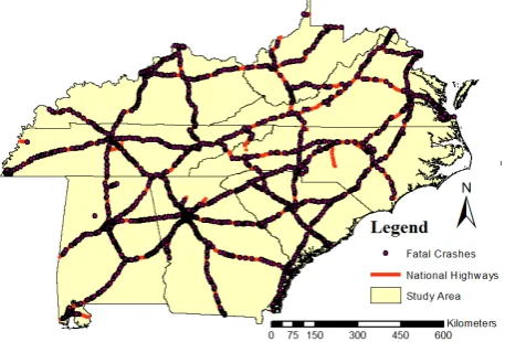
This study used the real world fatal crashes data occurred in several states in the east of US. This crashes were occurred on highways that connect eight states of Alabama, Georgia, North and South Carolina, Virginia, West Virginia, Kentucky, and Tennessee. Data used consist of the spatial and nonspatial data of fatal crashes occurred from beginning of 2007 to the end of 2009. During these years 2432 fatal crashes were recorded. Some of these crashes related to pedestrians’ crashes and some of them related to multi vehicle crashes. This study works on a part of data related to two vehicle crashes that includes 828 crashes (see Figures. 1 and 2). Table 1 shows the spatial and nonspatial variables used in this study.
Figure 1.Study area
Figure 2. Fatal crashes on US rural highways
light condition
Table 1.Spatial and nonspatial variables
2.2 Geographic weighted regression
As mentioned in the introduction, OLS method cannot be adapted
to features’ of spatial data because this method has assumed that data are completely independent and environment is homogenous. Hence, OLS method without considering dependency gives an answer for all points of reign and for this reason, a GWR method was presented by (Brunsdon et al., 1998). In this method, spatial dependency of observation is considered as the weight matrix due to environment homogeneity and non-stationarity regression coefficients were derived locally and separately for each point. The general relation for GWR is as follows (Brunsdon et al., 1998):
� = � , + ∑ � ,
= + � (1)
Where y is the dependent variable, Xj is the independent variable,
p is thenumber of independent variables, � is the residual of the model, and � is the coefficient of regression that is a function of observation point (u,v). Unlike OLS, the GWR is the weighted adjustment and the coefficients of regression can be computed by (Brunsdon et al., 1998):
�̂ , = , − , � (2)
where W is the weight matrix of observations that is a function of
[ , ⋱
, ] (3)
Determining the geographical weights is so important in GWR method. In this regard, several kernels have been presented for this purpose. In this study, the GWR method was used with two kernels that have demonstrated superior performances. The Gaussian and Tricube kernels are as follows (McMillen and McDonald, 2004):
= � �ℎ (4)
= {( − ℎ ) , ≤ ℎ
, > ℎ
(5)
Where is the geographic weight of observation j on the point
i, � is the normal standard distribution function, is the distance between two points i and j, and � is the standard deviation for for each point and h is the bandwidth. is the Euclidean distance in Cartesian coordinate when using geographic coordinates the distance is great circle distance. The most important issue in determining the geographic weights is selecting appropriate bandwidth because if this parameter is too large, GWR trends to OLS results and if too small bandwidth is selected, the variance will increase (Charlton and Fotheringham, 2009).
There are several method for optimizing bandwidth. One of them is Cross Validation method which can be computed by (Brunsdon et al., 1998):
∑ [� − �= ̂ ℎ ]� (6)
Where n is the number of observation, � is the observation i,and �̂ is the estimated value for the observation i computed by the other observations. Also, �̂ is a function of bandwidth and if bandwidth minimizes the function, it will be considered as the optimal bandwidth. Actually, in goodness of fit, determining the bandwidth is more effective than the kind of kernel used. There are two methods for selecting bandwidth (Charlton and Fotheringham, 2009):
• Fixed bandwidth: if data are distributed regularly, fixed bandwidth will be used.
• Unfixed (changeable) bandwidth: it is used in the cases that data are almost irregular and have clustered distribution. In this regard, in the high density area bandwidth decreases and vice versa. One criterion for this change can be the minimum and maximum of observation points in search band. Moreover, bandwidth can be changed in a way the fixed number of observations would stay on each band.
2.3 Evaluation Criteria
There are different parameters for evaluating the results of regression. One of them is R2 that indicates the goodness of fit for the achieved result. The value of R2 is between 0 and 1. R2 =0 indicates that using explanatory variables (effective parameters on crashes in this study) are not effective on estimating the dependent variable (the number of casualties in this study) and R2=1 indicates that the dependent variable is completely predictable using regression model. R2 can be calculated by(Shekhar and Xiong, 2007):
= − �
� (7)
�= ∑= � − �̂ (8)
= ∑= � − �̅ (9)
Where n is the number of observations, � is the value of dependent variable, i.e. observation, i, �̂ is the estimated value for the dependent variable, �̅ is the mean of observations. The methods that have been used for evaluation of residuals are RMSE and NRMSE that are computable by:
� = √ ∑= � − �̂ (10)
� = � ��
�̂ (11)
Where ��̂ is standard deviation for the estimated values of dependent variables.
3. IMPLEMENTATION
In this study, the number of casualties were considered as the dependent variable and the number of persons in crash, road alignment, number of lanes, pavement type, surface condition, road fence, light condition, vehicle type, weather, drunk driver, speed limitation, harmful event, road profile, and junction type were considered as explanatory variables. These factors were selected based on previous studies and our limitation to access the data.
Firstly, correlation between data must be checked by (Dale, 2014):
� , =∑�=1 − ̅ − ̅ (12)
� = � �� , (13)
Figure 3. Correlation matrix of explanatory variables
Table 2. The results of evaluation criteria for implemented algorithms
Figure 4 shows the result of OLS regression. The blue line depicts the actual data and the red line depicts the predicted result by the OLS.
Figure 4. Results of OLS regression
Figures 5 and 6 show the results of the proposed GWR using Gaussian and Tricube kernels, respectively. The blue line depicts actual data and the red line depicts the predicted result by GWR with kernels. In GWR both of bandwidth have been used and in order to optimize the bandwidth, the cross validation method was used. Moreover, Table 2 shows the achieved results for evaluation criteria used.
Figure5. Results of GWR with Gaussian kernel
Figure 6. Results of GWR with Tricube kernel
As shown in Table 2, R2 was calculated for both GWR and OLS the value of R2 for OLS has been obtained 0.0654 that is near zero. It implies that using explanatory variables (effective factors on crashes in this study) are not useful on estimating the dependent variable, i.e. the number of casualties. Hence, the OLS is not appropriate method for this issue while the calculated value for GWR with Gaussian kernel is 0.1294 and with Tricube kernel is 0.9196 that demonstrate better performance of GWR method in comparison with OLS for rural highway crashes. In fact OLS cannot be adapted with spatial autocorrelation and spatial non-stationarity because in this method, it was assumed that the data were completely independent and environment was homogenous. As a result, OLS without considering spatial dependency presented an answer for whole region. Furthermore, the obtained results for RMSE and NRMSE for GWR with Tricube kernel has great difference with both GWR with Gaussian kernel and OLS model therefor using GWR with Tricube kernel in rural highway crashes can improve accuracy and increase performance of detecting effective factors on rural highways crashes.
4. CONCLUSIONS
Today detecting effective factors of road accidents is so important because the number of passengers’ have been injured or died by driving accidents is too much. These casualty causes irreparable social and economical impacts. Hence, identifying hazardous times and places can be used in preventing future accidents’ occurrence. The goal of this paper is to develop an appropriate model for regression on rural highway crashes factors. Crashes are spatial events that occur in geographic space. The former regressions used for this purpose are not compatible with spatial data features like spatial autocorrelation and spatial non-stationarity. Thus, the GWR method as an appropriate
GWR OLS
Gaussian Tricube
R
2
R
M
S
E
NR
M
S
E
R
2
R
M
S
E
NR
M
S
E
R
2
R
M
S
E
NR
M
S
E
method for studying local patterns with adaptivity with spatial data features was used. For evaluation, the proposed method was applied to the real-world data of US rural highways recorded from 2007 to the end of 2009. In order to show the impact of spatial data features on regression, we compered the result of the proposed GWR method with that of OLS method. Goodness of fit result of OLS on highway crashes was 0.0654 while this value was 0.9196 for the proposed GWR method with Tricube kernel. As a result, using GWR with Tricube kernel can enhance accuracy and increase performance of detecting effective parameters on occurrence of crashes in rural highways.
In future study we recommend using combination of GWR with evolutionary algorithms to identify most effective factors on accidents. Also, using the GWR method with Tricube kernel in urban crashes is proposed in order to detect the effective factors of accidents in urban areas.
REFERENCES
Black, W.R., 1991. HIGHWAY ACCIDENTS: A SPATIAL AND TEMPORAL ANALYSIS. Transp. Res. Rec. Brunsdon, C., Fotheringham, S., Charlton, M., 1998.
Geographically weighted regression. J. R. Stat. Soc. Ser. Stat. 47, 431–443.
Chang, L.-Y., Chen, W.-C., 2005. Data mining of tree-based models to analyze freeway accident frequency. J. Safety Res. 36, 365–375.
Charlton, M., Fotheringham, A.S., 2009. Geographically weighted regression. White paper, National Centre for Geocomputation National University of Ireland Maynooth.
Chen, C., Zhang, G., Liu, X.C., Ci, Y., Huang, H., Ma, J., Chen, Y., Guan, H., 2016. Driver injury severity outcome analysis in rural interstate highway crashes: a two-level Bayesian logistic regression interpretation. Accid. Anal. Prev. 97, 69–78. doi:10.1016/j.aap.2016.07.031 Clarke, D.D., Forsyth, R., Wright, R., 1998. Machine learning in
road accident research: decision trees describing road accidents during cross-flow turns. Ergonomics 41, 1060–1079.
Dale, P., 2014. Mathematical Techniques in GIS. CRC Press. de Oña, J., López, G., Mujalli, R., Calvo, F.J., 2013. Analysis of
traffic accidents on rural highways using Latent Class Clustering and Bayesian Networks. Accid. Anal. Prev. 51, 1–10. doi:10.1016/j.aap.2012.10.016
Delen, D., Sharda, R., Bessonov, M., 2006. Identifying significant predictors of injury severity in traffic accidents using a series of artificial neural networks. Accid. Anal. Prev. 38, 434–444.
Kashani, A.T., Mohaymany, A.S., 2011. Analysis of the traffic injury severity on two-lane, two-way rural roads based on classification tree models. Saf. Sci. 49, 1314–1320. McMillen, D.P., McDonald, J.F., 2004. Locally weighted maximum likelihood estimation: Monte Carlo evidence and an application, in: Advances in Spatial Econometrics. Springer, pp. 225–239.
Pakgohar, A., Tabrizi, R.S., Khalili, M., Esmaeili, A., 2011. The role of human factor in incidence and severity of road crashes based on the CART and LR regression: a data mining approach. Procedia Comput. Sci. 3, 764–769. PARK, S.H., KIM, D.-K., KHO, S.-Y., RHEE, S., 2010.
Identifying hazardous locations based on severity scores of highway crashes, in: 12th World Conference on Transport Research, Lisbon.
Rhee, K.-A., Kim, J.-K., Lee, Y., Ulfarsson, G.F., 2016. Spatial regression analysis of traffic crashes in Seoul. Accid.
Anal. Prev. 91, 190–199.
doi:10.1016/j.aap.2016.02.023
Shekhar, S., Xiong, H., 2007. Encyclopedia of GIS. Springer Science & Business Media.
Sohn, S.Y., Shin, H., 2001. Pattern recognition for road traffic accident severity in Korea. Ergonomics 44, 107–117. Tobler, W.R., 1970. A Computer Movie Simulating Urban
Growth in the Detroit Region. Econ. Geogr. 46, 234– 240. doi:10.2307/143141
Xu, P., Huang, H., 2015. Modeling crash spatial heterogeneity: Random parameter versus geographically weighting. Accid. Anal. Prev. 75, 16–25. doi:10.1016/j.aap.2014.10.020