Vol. 43 (2000) 167–198
A contribution to the evolutionary theory of
innovation, imitation and growth
q
Katsuhito Iwai
∗Faculty of Economics, The University of Tokyo, Hongo 7-3-1, Bunkyo-ku, Tokyo 113-0033, Japan
Received 11 January 1999; received in revised form 4 April 2000; accepted 5 April 2000
Abstract
This paper develops mathematically tractable evolutionary models that can be used to analyze the development of industrial structure as a dynamic process moved by complex interactions among innovations, imitations and investments of satisficing firms striving for survival and growth. It demonstrates that what the industry will approach in the long-run is not a neoclassical equilibrium of uniform technology but at best a statistical equilibrium of technological disequilibria which maintains a relative dispersion of efficiencies in a statistically balanced form. This paper also shows that these evolutionary models can simulate all the macroscopic characteristics of neoclassical growth models without assuming the full rationality of business behavior. © 2000 Elsevier Science B.V. All rights reserved.
JEL classification: L10; O30; D50; P10
Keywords: Evolutionary economics; Schumpeter; Disequilibrium; Technological change; Growth accounting
1. Introduction
“Capitalist economy is not and cannot be stationary,” said Joseph Schumpeter more than half a century ago (1950, p. 31). “Stationary socialism is still socialism but stationary capitalism is impossible, is, in fact, a contradiction in terms” (1946, p. 198).
q
This paper was originally circulated under the title of “Towards a disequilibrium theory of long-run profits”. An earlier version of this paper was presented at ISER XI Workshop at the Certosa di Pontignano, Siena, on 1 July 1998. I am grateful to the participants of the Workshop for their helpful comments and suggestions. I have also benefited from useful suggestions of a referee and an editor of this journal. The remaining errors are, of course, mine.
∗Tel.:+81-3-3812-2111; fax:+81-3-3818-7082.
E-mail address: [email protected] (K. Iwai).
Nevertheless, Schumpeter (1939, p. 49) claimed, traditional economic theory, be it classi-cal or neoclassiclassi-cal, is primarily the theory of the stationary process — of the process which “merely reproduces at constant rates and is in equilibrium at every point of time.” This does not mean that the traditional theory cannot cope with fluctuations and growth. It can describe business fluctuations as adaptive adjustments of equilibrium state in response to external disturbances; it can explain economic growth as a steady movement of equilibrium state in response to increase in population and accumulation of savings. In particular, the accumulation of savings plays a large role in the traditional account of economic growth. But, argued Schumpeter, it “owes its quantitative importance to another factor of change without which its modus operandi in the capitalist world cannot be understood” (p. 59). And this “another factor of change” is, of course, what Schumpeter called “innovation” — a broad range of events which includes “the introduction of new commodities, etc., the technological change in the production of commodities already in use, the opening-up of new markets or of new sources of supply, Taylorization of work, improved handling of material, the setting-up of new business organizations, etc. — in short, any ‘doing things differently’ in the realm of economic life” (p. 59).
In the conditions of a stationary or even of a steadily growing economy, Schumpeter maintained, “the bulk of what is in common parlance described as profits” would vanish if earnings of management and various interest items are counted as costs (p. 80). And the function of innovation is precisely to destroy this stalemate of classical and neoclas-sical equilibrium by endowing the innovator with a power to raise the price above the prevailing cost or to lower the cost below the prevailing price. “Profit” is thus “the pre-mium put upon successful innovation in capitalist society” (pp. 79–80). But the innovator’s price–cost advantage does not last forever. Once an innovation is successfully introduced into the economy, “it becomes much easier for other people to do the same thing” (p. 75). A subsequent wave of imitations renders the original innovation obsolete and gradually diminishes the innovator’s profit margin. And yet, Schumpeter argued, the characteristic feature of “disequilibria” created by innovations is that “they recur with some regularity” (p. 72). For “there will always be possibilities for new combinations [i.e., innovations]. . .
, and always some people able and willing to carry them out” (p. 105). Capitalist economy indeed consists in the “process of creative destruction” that “incessantly revolutionalizes the economic structure from within, incessantly destroying an old one, incessantly creating a new one” (1950, p. 83).
The purpose of this paper is to formalize some of the essential features of the capitalist economy from the perspective of ‘evolutionary economics’.1 Indeed, Schumpeter (1939, p. 74) was one of the first to challenge the assumption of perfect rationality of human decision-makings in traditional economic theory. He said that “the assumption that business behavior is ideally rational and prompt. . .works tolerably well only within the precincts of tried experience and familiar motive,” and then claimed that “it breaks down as soon as we leave those precincts and allow people to be faced by new possibilities of business action which are as yet untried and about which the most complete command of routine teaches
nothing.” In the present paper I will present a series of ‘simple evolutionary models’ that can describe the development of an industry’s state of technology as an aggregate outcome of dynamic interactions among innovations, imitations and growth at the micro-level of firms. These models are ‘evolutionary’ because they assume that the firms’ innovative, imitative and growth activities are guided not by optimizing policies based on rational calculations but by satisficing behaviors based on organizational routines.2 These models are ‘simple’ because they allow us to characterize, only by pencils and paper, both the short-run movement and long-run performance of the industry’s state of technology in closed-form expressions.
Mathematically tractable and yet empirically plausible evolutionary models have been very scarce because of the intrinsic difficulty in formalizing dynamic models without the help of optimization technique and equilibrium concept. In fact, most evolutionary economic models have had to rely on numerical simulations for their analyses, thereby casting doubt on their general applicability. It is hoped that just to present a series of evolutionary models that are simple enough to allow closed-form solutions will be a net addition to the recently emerged and rapidly expanding discipline of evolutionary economics.3
This paper is organized as follows. The rest is divided into two sections. Section 2 presents the basics of our simple evolutionary models. After setting up the static structure of the industry’s technology in Section 2.1, Sections 2.2 and 2.3 examine how firms’ imitative and innovative activities move the state of technology over time. It is argued that while the swarm-like appearance of imitations pushes the state of technology towards uniformity (hence the economic evolution has a Lamarkian feature), the punctuated appearance of innovations disrupts the imitations’ equilibriating tendency. Section 2.4 then turns to the long-run of the industry’s state of technology. It shows how these conflicting microscopic forces will balance with each other in a statistical sense and give rise to a long-run average distribution of efficiencies across firms. What the economy approaches in the long-run is not a classical and neoclassical equilibrium of uniform technology but at best a statistical equilibrium of technological disequilibria.
The central core of any evolutionary theory worthy of the name is the Darwinian selection mechanism — the fittest survives and spreads its favored traits through higher reproduction rate. In the case of economic evolutionary models, this selection mechanism works itself out through differential growth rates between high profit firms and low profit firms (or between high profit capital stocks and low profit capital stocks). In order to incorporate this mechanism, Section 3 of the paper superimposes the process of capital growth upon the evolutionary models of Section 2. In fact, Section 3.1 sets up two alternative models of capital growth — one for disembodied technology and the other for embodied technology. Sections 3.2 and 3.3 then analyze the dynamic interactions between capital growth on the one hand and technological imitations and innovations on the other and then derive the
2The term “satisficing” designates the behavior of a decision maker who does not optimize a well-defined objective function but simply seeks to obtain a satisfactory utility or return. See Simon (1957).
long-run average efficiency distributions of capital stocks. Even if the Darwinian selection mechanism is introduced explicitly into our picture of the economy, what it will approach in the long-run is still not a classical and neoclassical equilibrium of uniform technology but at best a statistical equilibrium of technological disequilibria which reproduces a relative dispersion of efficiencies among capital stocks in a statistically balanced form.
The challenge to any theory claiming to challenge the traditional theory is to match its power to predict the empirical patterns of the developmental processes of advanced capital-ist economies. The purpose of the penultimate section (Section 3.4) is indeed to demonstrate that our simple evolutionary models are capable of ‘simulating’ all the macroscopic char-acteristics of neoclassical growth model both in the short-run and in the long-run.4 If
the neoclassical growth model is capable of accounting the actual developmental paths of advanced capitalist economies, our simple evolutionary models are equally capable of performing the same task. Section 3.5 concludes the paper.
2. An evolutionary model of imitation and innovation
2.1. The state of technology in the short-run
Consider an industry which consists of a large number of firms competing with each other. Some firms are active participants of the industry, busy turning out products; others are temporarily staying away from production but are ready to start it when the right time comes. Let us denote by F the total number of firms, both active and inactive, and assume it to be constant over time. In order to make the description of the industry as general as possible at this stage of analysis, I will not specify the market structure until Section 3.1; the industry may face a perfectly competitive market or a monopolistically competitive market or other market form for its products.
The starting point of our evolutionary model is an observation that technological knowl-edge is not a pure public good freely available among firms at least in the short-run. Ac-cordingly, let us suppose that there are Nt distinct technologies in an industry at time t, which can be labeled as 1,2, . . . , Nt −1, Nt. Let us also suppose that their efficiency can be ordered linearly from the worst to the best, so that we can identify the index 1 as the least efficient and the index Ntas the most efficient technology. In Section 2.3 I will specify these technologies in more detail, but until then there is no need to commit to any particular specification. Note that the index of the best technology Nt has a time subscript t, because firms’ innovative activities are bringing in new technologies into the industry every now and then, as we will soon see.
Let me describe how technologies are distributed over firms, or it comes to the same thing, how firms are distributed over technologies. For this purpose, let ft(n) stand for the relative share of firms having access to the nth technology at time t. (Their total number is equal to
Fft(n).) It of course satisfies an adding-up equation:ft(1)+ · · · +ft(n)+ · · · +ft(Nt)=1. The set of these shares,{ft(n)}, is called the ‘efficiency distribution of firms’ at time t, for it gives us a snap-shot picture of the distribution of firms over a spectrum of technologies
from the best to the worst. Unlike the paradigm of classical and neoclassical economics, however, the state of technology is never static in a capitalist economy. As time goes by, dynamic competition among firms over technological superiority constantly changes the efficiency distribution of firms from one configuration to another. I will now turn to the evolutionary process of the efficiency distribution of firms in our Schumpeterian industry.
2.2. Imitations and the evolution of the state of technology
There are basically two means by which a firm can advance its technology — by inno-vation and by imitation. A firm may succeed in putting a new and better technology into practice by its own R&D efforts. A firm may increase its efficiency by successfully copying another firm’s technology. The evolution of the state of technology is then determined by the dynamic interaction of innovations and imitations. We take up the process of imitations first.
Technological information is not a pure public good freely available among firms. It is, however, not a pure private good either. As remarked by Arrow (1962, p. 615), “the very use of the information in any productive way is bound to reveal it, at least in part”, and “mobility of personnel among firms provides a way of spreading information.” Even if property rights are assigned to the owners of new technology, they can provide only a partial barrier, “since there are obviously enormous difficulties in defining in any sharp way an item of information and differentiating it from other similar sounding items.” New technology is bound to spread among firms through their imitative activities and its secret is more likely to leak out as more and more firms have come to use it for production. There is always an element of bandwagon effect in the diffusion of new ideas or new things (e.g., Coleman et al., 1957). The following hypothesis formalizes such a diffusion process in the simplest possible manner.5
Hypothesis (IM-b). Firms seek to imitate only the best technology Nt, and the probability that one of the firms succeeds in imitating the best technology during a small time interval dt is equal toµFft(Nt)dt, where Fft(Nt) is the number of firms currently using the best technology andµ(>0) is a small constant uniform across firms.
The imitation parameterµrepresents the effectiveness of each firm’s imitative activity. As was indicated in Section 2.1, the present paper follows the strict evolutionary perspective in supposing that firms do not optimize but only “satisfice” in the sense that they simply follow organizational routines in deciding their imitative, innovative and growth policies. Indeed, one of the purposes of this paper is to see how far we can go in our description of the economy in dynamic performances without the assumption of individual super-rationality. We simply assumeµas a given constant whose value is a legacy from the past.
5Both Hypotheses (IM′) and (IM) in Iwai (1984a,b, 1998) suppose that firms imitate not only the best technology
but also any of the technologies better than the ones currently used. Hypothesis (IM′) then assumed that the
probability of imitating the nth technology is equal toµft(n) per unit of time and Hypothesis (IM) then assumed
that the probability is equal toµst(n), where st(n) represents the capital share of the nth technology. Note thatµF
Hypothesis (IM-b) allows us to analyze the evolution of the efficiency distribution of firms in the following manner. First, consider the evolution of the share of the best technology firms ft(Nt). Its value increases whenever one of the firms using a lesser technology succeeds in imitating the best technology Nt. Since the relative share of those firms is 1−ft(Nt)and the probability of such a success for each firm isµFft(Nt)dtduring a small interval dt, we can calculate the expected increase in ft(Nt) during dt as(µFft(Nt)dt )(1−ft(Nt)). If the number of firms F is sufficiently large, we can apply the law of large numbers and deduce the following differential equation (as a good approximation) for the actual rate of change in ft(Nt):
˙
ft(Nt)=µFft(Nt)(1−ft(Nt)). (1)
This is of course a ‘logistic differential equation’ with a logistic parameterµF. Setting T
as an initial time, it is not hard to solve it to obtain the following explicit formula:6
ft(Nt)=
1
1+(1/fT(Nt)−1)e−µF (t−T )
for t ≥T , (2)
where e stands for the exponential. This is nothing but a ‘logistic growth curve’ which appears frequently in population biology and mathematical ecology.
Next, consider the evolution of the relative share of the firms employing one of the less efficient technologies or of ft(n) forn=Nt−1, Nt−2, . . . ,1. This share decreases when-ever one of those firms succeeds in imitating the best technology. Since the relative share of those firms is ft(n) and the probability of such a success for each firm isµFft(Nt)dtduring a time interval dt, we can calculate the expected decrease in ft(n) as(µFft(Nt)dt )ft(n). The law of large numbers then enables us to deduce the following differential equation (as a good approximation) for the actual rate of change in ft(n):
˙
ft(n)= −µFft(Nt)ft(n), n=1,2, . . . , Nt−1. (3)
We can also solve this to obtain the following formulae:
ft(n)=
fT(n)(1−ft(Nt)) 1−fT(Nt)
, n=1,2, . . . , Nt−1 (4)
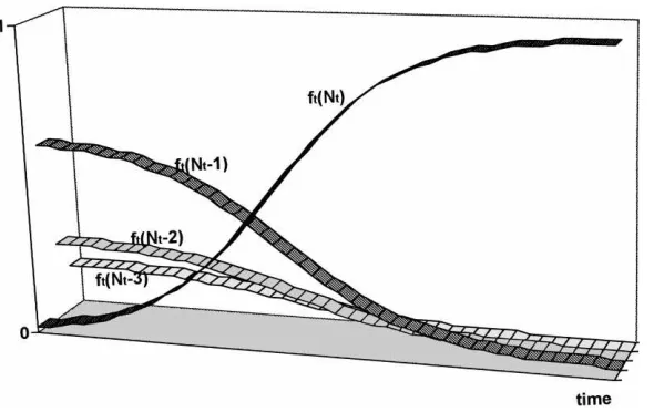
fort ≥T. They describe the way the shares of the lesser technology decay over time. Fig. 1 illustrates the evolution of both growth equation (2) and decay equation (4) in a three-dimensional diagram. Its x-axis measures time, y-axis the technology index, and
z-axis the share of firms. The S-shaped curve in the front traces the growth pattern of the
share of the best technology firms. Every other curve traces the decaying pattern of the share of each of the lesser technology firms. These curves give us a motion picture of the evolution of the state of technology, {ft(Nt), . . . , f (1)}, under the pressure of imitative activities. When only a small fraction of firms use the best technology, imitation is difficult and the growth of its users is slow. But one imitation breeds another and a bandwagon soon
6A logistic differential equationx′=ax(1−x)can be solved as follows. Rewrite it asx′/x−(1−x)′/(1−x)
and integrating it with respect to t, we obtain logx−log(1−x)=logx0−log(1−x0)+at, or x/(1−x)= eatx
Fig. 1. Evolution of the efficiency distribution of firms under the sole pressure of technological diffusion.
sets in motion. The growth of the share of the best technology accelerates until half of the firms come to adopt it. Then the growth starts decelerating, while the share itself continues to grow until it absorbs the whole population in the industry. In the long-run, therefore, the best technology will dominate the entire industry. Such swarm-like process of technological diffusion is nothing but an economic analog of the “Lamarkian” evolutionary process.
2.3. Innovations and the evolution of the state of technology
Does this mean that the industry’s long-run state is no more than the paradigm of classical and neoclassical economics where every market participant has complete access to the best technology available in the industry? The answer is a “No”. And the key to this answer lies in the innovation — the carrying out of what Schumpeter called a “new combination”. Indeed, the function of innovative activities is precisely to destroy this evolutionary tendency towards a static equilibrium.
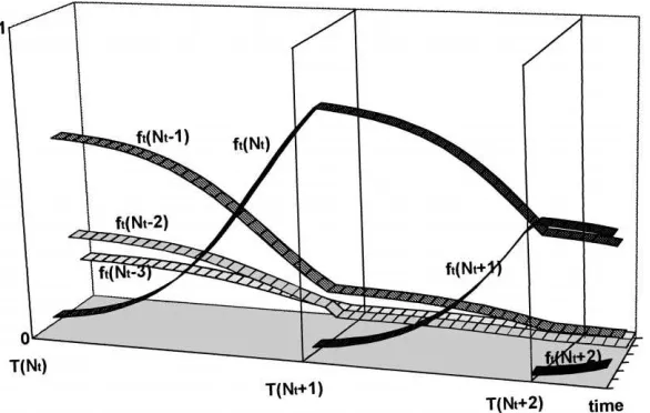
Suppose that at some point in time, one of the firms succeeds in introducing a new and better technology into the industry. From that time onwards, this new technology takes over the best technology index Ntand the former best technology is demoted to the lesser index
Nt−1. Let us denote this epoch by T(Nt) and call it the ‘innovation time’ for Nt. Since the total number of firms is F, this means that att =T (Nt)a new share ft(Nt) emerges out of nothing and takes the value of 1/F.
No sooner does this innovation take place than do all the lesser technology firms seek the opportunities to imitate it. Under Hypothesis (IM-b), this sets in motion a new logistic growth curve (2) of ft(Nt) from an initial share 1/F. Hence, we have
ft(Nt)=
1
Fig. 2. Evolution of the efficiency distribution of firms under the joint pressure of technological diffusion and recurrent innovations.
As for the lesser technologies (including the former best technology which now has the index ofNt−1), each of their shares then follows a decay curve (4), or
ft(n)=
fT (Nt)(n)(1−ft(Nt))
1−1/F for t≥T (Nt), n=1,2, . . . , Nt−1. (6)
Note here that if the innovator used technology m just before the innovation, the share ft(m) loses 1/F att=T (Nt). But all the other shares traverse the innovation time T(Nt) without any discontinuity. Fig. 2 squeezes all these processes into a three-dimensional diagram.
Innovation is not a single-shot phenomenon, however. No sooner than an innovation takes place, a new round of competition for a better technology begins, and no sooner than a new winner of this game is named, another round of technological competition is set out. The whole picture of Fig. 2 exhibits how the industry’s state of technology evolves over time as a dynamic interplay between two opposing technological forces — swarm-like appearance of imitations and creative destruction of innovations. While the former works as an equilibriating force which tends the state of technology towards uniformity, the latter works as a disequilibriating force which destroys this leveling tendency.
A new question arises: is it possible to derive any law-like properties about the industry’s state of technology out of this seemingly erratic movement? In order to give an answer to this question, we need to characterize the nature of technological innovations in more detail. The next hypothesis is about the impact of each innovation on the rate of productivity increase.
Hypothesis (PG). Each innovation causes the productivity of the industry’s best technology
If we denote by a(n) the labor productivity of the nth innovation, then it is given by eλn
. The next assumption is about the stochastic nature of the way innovations take place over time. Indeed, this paper presents two alternative hypotheses.
Hypothesis (IN-a). Every firm has an equal chance for an innovation, and the probability
that each firm succeeds in an innovation during a small time interval dt isνdt, whereν(>0) is a constant much smaller thanµand uniform across firms.
Hypothesis (IN-b). Only the firms using the best technology are able to carry out the next
innovation, and the probability that each of these firms succeeds in an innovation during a small time interval dt isξdt, whereξ(>0) is a constant much smaller thanµand uniform across firms.
The above two hypotheses constitute two polar cases about the pool of potential innovators from which the next innovator is drawn. Hypothesis (IN-a) insists that there is no prerequisite knowledge for a firm to become an innovator, whereas Hypothesis (IN-b) insists that one has to practice the most advanced technology in order to make a further progress on it. The reality of course lies somewhere in between.
The innovation parameterν orξ represents the effectiveness of each firm’s innovative activity. In the present paper which has adopted a strict evolutionary perspective, their values are taken as exogenously given. Since the total number of firms is F, Hypothesis (IN-a) implies that the probability of an innovation during a small time interval dt is given byνFdt. Since the total number of best technology firms is Fft(Nt), Hypothesis (IN-b) implies that the probability of an innovation during a small time interval dt is given by
ξFft(Nt)dt.
We have already defined T(Nt) as the time at which a technology Nt is introduced for the first time into an industry. A difference between two adjacent innovation times,T (Nt+ 1)−T (Nt), thus defines a ‘waiting period’ for the next innovation. Let W(t) denote its probability distribution, orW (t )≡Pr{T (Nt+1)−T (Nt)≤t}. Then, Appendix A shows that it can be expressed asW (t ) = 1−e−νFt under Hypothesis (IN-a) and asW (t ) = 1−(((F−1)+eµFt)/F )−ξ /µunder Hypothesis (IN-b). Letωdenote the ‘expected waiting time’ of the next innovation, orω≡E(T (Nt+1)−T (Nt))=R0∞tdW (t ). Then, Appendix A also shows that it can be calculated as
ω= 1
νF (7a)
under Hypothesis (IN-a), and as
ω=
∞
X
i=0
(1−1/F )i
(ξ+µi)F (7b)
under Hypothesis (IN-a). Note that an increase inνdecreasesωof (7a) and an increase in
2.4. The efficiency distribution of firms in the long-run
The state of technology given by{ft(n)}is a historical outcome of the dynamic interaction between imitations and innovations. A swarm-like appearance of imitations is an equilibri-ating force which pushes the industry’s state of technology towards uniformity, whereas the punctuated arrival of an innovation is a disequilibrium force which destroys such tendency towards technological uniformity. Every time an innovation has taken place, a new round of imitative activities starts from scratch and resumes their pressure towards technological uniformity. As time goes by, however, innovations turn up over and over again and reset the process of imitations over and over again. In fact, under both Hypotheses (IN-a) and (IN-b), the sequence of waiting periods are mutually independent random variables having the same probability distribution W(t), so that the whole movement of{ft(n)}within each waiting period becomes a statistical replica of each other. This means that the entire evolutionary process of the state of technology now constitutes what is called a “renewal process” in the probability theory.7 (As a matter of fact, under Hypothesis (IN-a) it constitutes the sim-plest of all renewal processes — a “Poisson process”.) We can thus expect that over a long passage of time, a certain statistical regularity will emerge out of its seemingly irregular patterns.
The first regularity we want to examine is about the productivity growth rate of the best technology. For this purpose let us note that Nt, the index of the best technology at time
t, can also be identified with the number of innovations occurring from time 0 to time t.
Then the so-called ‘renewal theorem’ in the probability theory as in Feller (1966, p. 137) says that as t becomes very large, the random occurrence of innovations will be gradually averaged out and that the expected rate of innovations E(Nt)/t will approach the inverse of the expected waiting period 1/ω. Since by Hypothesis (PG), each innovation raises the productivity by a rateλ, the productivity of the industry’s best technology is thus expected to grow at the rate ofλ/ωin the long-run. Hence by (7a), we have
E
log(a(N t))
t
→νF λ (8a)
under Hypothesis (IN-a), and by (7b), we have
E
log(a(N t))
t
→ P F λ
i((1−1/F )i/(ξ+µi))
(8b)
under Hypothesis (IN-b). It is not hard to show that under Hypothesis (IN-a), an increase in
νandλincreases the long-run growth rate of the best technology, and that under Hypothesis (IN-b), an increase inξ,µandλincreases the long-run growth rate of the best technology.
The industry’s productivity growth is thus endogenously determined in this evolutionary model.8
Indeed, not merely the process of innovations but also the entire evolution of the effi-ciency distribution of firms is expected to exhibit a statistical regularity in the long-run. To see this, let us focus on the sequence of technology indices arranged in reverse order,
Nt, Nt −1, . . . , Nt −i, . . .. As t moves forward, a technology occupying each of these indices becomes better and better. But the best technology Nt is always the best technol-ogy, the second-best technology Nt−1 the second-best,. . ., the (i+1)th-best technology
Nt−i the (i+1)th-best, independent of their actual occupants. The set of technology shares, {ft(Nt), ft(Nt−1), . . . , ft(Nt−i), . . .}, thus represents the relative form of the efficiency distribution of firms. If there is any statistical regularity at all, it must come out from the re-current pattern of this relative distribution over a long passage of time. Let us thus determine its long-run average configuration.
Here I am omitting all the mathematical details and only reporting the results obtained in Appendix B first in the form of geometry and then in the form of algebraic equations.
Fig. 3a below illustrates the relative form of long-run average efficiency distribution when every firm can innovate, and Fig. 3b the relative form of the long-run average state of technology when only the best technology firms can innovate. The former has the form of geometric distribution, and the latter usually has a peak at the second-best technology and assumes the form of geometric distribution from that point onwards.
The mathematical formulae for these curves are given as follows. Under Hypothesis (IN-a), we have
We have thus seen that what our Schumpeterian industry approaches in the long-run is not a classical or neoclassical equilibrium of uniform technology but a statistical equilibrium
Fig. 3. Long-run average efficiency distribution of firms, (a) when every firm can strike an innovation and (b) when only one of the best technology firms can strike an innovation.
of technological disequilibria which reproduces a relative dispersion of efficiencies among firms in a statistically balanced form.
3. An evolutionary model of capital accumulation and technological change
3.1. The mechanism of economic selection
Let us denote by kt(n) the total capital stock carrying technology n at time t and by
Kt the total capital stock accumulated in the entire industry at time t. We of course have
Kt = kt(Nt)+kt(Nt −1)+ · · · +kt(1). Let us also denote by st(n) the ‘capital share’ of the nth technology at time t defined by kt(n)/Kt. We then call the set of capital shares,
{st(n)}, the ‘efficiency distribution of capital stocks,’ for it gives us a snapshot picture of the way the industry’s total capital stock is distributed over a spectrum of technologies from the most efficient to the least efficient. As is the case of efficiency distribution of firms
{ft(n)}, the efficiency distribution of capital stocks{st(n)}is never static in a capitalistic economy. Differential growth rates between efficient and inefficient capital stocks as well as technological competition among firms constantly change its configuration over time. In order to analyze this process, we now have to specify the structure of the markets as well as the structure of each technology much more concretely than in Section 2.
First, let us assume that each technology is of Leontief-type fixed proportion technology with labor service as the variable input and capital stock as the fixed input. Let us also assume that only the labor productivity varies across technologies so that the nth technology can be written as
y=Min[a(n)l,bk], (10)
where y, l and k denote output, labor and capital, and a(n) and b denote labor productivity and capital productivity, respectively. Because of Hypothesis (PG), we havea(n) =eλn, but b is assumed to be constant over time and uniform across technologies.
Next, let us also suppose that every firm in the industry produces the same product and hires homogeneous workers. They thus face the same price Ptfor the products they produce and the same money wage rate Wt for the workers they hire. Let rt(n) denote the real rate of profit (in terms of product price) accruing from the use of the nth technology at time
t. If the price of capital equipment is equal to the price of product, it can be calculated as
rt(n)=(Pty−Wtl)/Ptk=b(1−(Wt/Pt)/a(n)), which we approximate asb(log(a(n))− log(Wt/Pt))for analytical convenience. This is not a bad approximation as long as the labor productivity a(n) and the real wage rate Wt/Pt are not so wide apart. Sincea(n)=eλn, this can be further rewritten asb(λn−log(Wt/Pt)).
“Without development there is no profit, without profit no development”, so said Schum-peter (1961, p. 154). “For the capitalist system. . . without profit, there would be no ac-cumulation of wealth.” Our next step is to relate the firms’ capital growth policy to the rate of profit. Here, I would like to introduce two alternative hypotheses — one for the case of disembodied technology and the other for the case of embodied technology. In the case of disembodied technology all the capital stocks accumulated in a firm have the same productivity, whereas in the case of embodied technology different capital stocks may carry different technologies even in the same firm. We have the following hypotheses.
Hypothesis (CG-d). Technology is not embodied in capital stocks, and the growth rate of
a firm possessing nth technology is given byγ rt(n)−γ0, whereγ (>0) andγ0(>0) are
given positive constants uniform across firms.
Hypothesis (CG-e). Technology is embodied in capital stocks and the growth rate of capital
stocks embodying nth technology is given byγ rt(n)−γ0, whereγ (>0) andγ0(>0) are
Each of the above hypotheses tries to capture the Darwinian mechanism of economic selection in the simplest possible manner — capital stocks earning higher profit rates grow faster than the others and enlarge the shares of the technology they use. The parameterγ
represents the sensitivity of the firms’ growth rate to the rate of profits, and the parameter
γ0represents the rate of capital depreciation of the break-even firm or break-even capital
stock. Their values are taken as exogenously given in the present paper.
Now, all the hypotheses in our evolutionary models are finally laid out. First, Hypothesis (IM-b) concerning the spill-over effects of the best technology through imitations. Second, Hypothesis (PG) concerning the step-by-step process of innovations. Third, Hypotheses (IN-a) and (IN-b) concerning the nature of the pool of potential innovators and their success probability — the one supposing that every firm has an equal chance for innovation and the other supposing that only the best technology firms can innovate. And finally, Hypotheses (CG-d) and (CG-e) concerning firms’ capital accumulation policy — the one for the case of disembodied technology and the other for the case of embodied technology. We are now in a position to analyze how do these microscopic forces combine with each other and move the entirety of the efficiency distribution of capital stocks{st(n)}over time. It is necessary to proceed one by one.
In the first place, let us ignore both technological imitations and technological innovations for the time being so as to place the process of economic selection in full relief. Let us note that both Hypotheses (CG-d) and (CG-e) imply that the growth rate of capital stock with technology n can be expressed as
˙ of the growth rate of capital share as
˙
we then obtain the following set of differential equations for each of the capital shares
{st(n)}:
˙
st(Nt)=(γ λζt)st(Nt)(1−st(Nt)), (12)
˙
Fig. 4. Evolution of the efficiency distribution of capital stocks under the sole pressure of economic selection.
whereζtrepresents the gap between the best technology index and the average index of all the rest and is defined by
ζt ≡Nt − Nt−1
X
n
nst(Nt) 1−st(Nt)
. (14)
The value ofζt in general depends on t, but is expected to move only slowly over time.9 Indeed, for the sake of expositional simplicity, we will from now on proceed as if it were actually an exogenously given constantζ. Then, (12) takes the same logistic form as (1), and (13) the same mathematical form as (2) except for an additional term−(γ λ)(i−ζ )st(Nt−i). We can thus solve them to obtain
st(Nt)=
1
1+(1/sT (Nt)−1)exp{−γ λζ F (t−T (Nt))}
, (15)
st(Nt −i) =exp{−γ λ(i−ζ )(t−T (Nt))}
1−st(Nt) 1−sT (Nt)(Nt)
sT (N )(Nt −i),
i =1, . . . , Nt −1 (16)
forT (Nt)≤t.
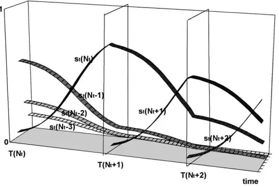
Fig. 4 illustrates the movement of the whole set of capital shares{st(Nt−i)}under the sole pressure of economic selection in a three-dimensional diagram whose x-axis measures time, z-axis technology index, and y-axis capital shares. It looks very much like Fig. 1, which illustrated the diffusion process of the best technology among firms. In fact, we have again encountered a now familiar S-shaped logistic growth curve, this time tracing out the
motion of the best technology’s capital share st(Nt). Yet, the logic behind Fig. 4 is entirely different from that of Fig. 1. In contrast to the Lamarkian evolutionary process depicted in Fig. 1, what Fig. 4 illustrates is a Darwinian evolutionary process which constantly shifts the distribution of capital shares from the lesser technology to the best technology through the relative difference in their growth rates. When the capital share of the best technology is very small, that share can grow almost exponentially by constantly absorbing the shares of the lesser technologies. But as the best technology begins to occupy a larger and larger capital share, the shares of the lesser technologies it absorbs become smaller and smaller. It thus gradually loses its growth momentum, but keeps growing nevertheless until it finally swallows the whole industry. If there is neither technological imitation nor technological innovation, only the fittest will survive in the long-run state of the industry, and this of course reproduces the Darwinian mechanism of natural selection in the world of economics.
3.2. Capital growth and technological diffusion
In our Schumpeterian industry, there is a continuous wave of technological imitations as well as an intermittent arrival of technological innovations incessantly interfering the way capital stocks are accumulated over time. We thus have to modify the economic selection process discussed in the preceding section in order to take account of such technological interference. In the present section I will re-introduce the process of technological diffusion, leaving the re-introduction of technological innovations to the next section.
As we will now see, the impact of technological imitations on capital accumulation is different when it is embodied in capital stocks and when it is not. Let me examine the case of disembodied technology first.
Now, we know from (1) that under Hypothesis (IM-b) Ff˙t(Nt) = µF2ft(Nt)(1−
ft(Nt))firms succeed in imitating the best technology Nt during each time unit. In the case of disembodied technology, these firms can transform all their capital stocks into the most efficient ones. Since their average capital share is(1−st(Nt))/F (1−ft(Nt)), their successful imitations on average increase the best technology’s capital share st(Nt) by
1−st(Nt)
F (1−ft(Nt))
µF2ft(Nt)(1−ft(Nt))=µFft(Nt)(1−st(Nt)). Adding this to the right-hand side of (12), we have
˙
st(Nt)=(γ λζ st(Nt)+µFft(Nt))(1−st(Nt)) (17d)
for T (Nt) ≤ t < T (Nt +1). By the same token, we know from (2) that−Ff˙t(Nt −
i) = −µF2ft(Nt)ft(Nt −i) firms abandon technology Nt −i by imitating the best technology Ntduring each time unit. Since the average capital share of these firms is equal to
st(Nt−i)/Fft(Nt−i),they on average subtract
µF2ft(Nt)ft(Nt−i)st(Nt−i)
Fft(Nt−i)
=µFf(Nt)st(Nt−i)
from the right-hand side of (13). Hence, under both Hypotheses (CG-d) and (IM-b), we have
˙
st(Nt −i) = −(γ λζ st(Nt)+γ λ(i−ζ )+µFft(Nt))st(Nt−i),
forT (Nt)≤t < T (Nt+1). As will be shown in Appendix C, it is possible to solve these two differential equations and derive (after some hard work) the following rather formidable expressions:
st(Nt)=1−
Ψ (ft(Nt))
(1/(1−sT (Nt)))−(γ λζ /µF )
Rft(Nt)
1/F Ψ (x)dx
, (19d)
whereΨ (x) ≡(x/(1/F ))−γ λζ /µF((1−x)/(1−1/F ))1+γ λζ /µF, and ft(Nt) is a logistic curve 1/(1+(F−1)eµF (t−T (Nt)))defined by (5);
st(Nt −i) =exp{−γ λ(i−ζ )(t−T (Nt))}
1−st(Nt) 1−sT (Nt)(Nt)
sT (Nt)(Nt −i),
i =1,2, . . . , Nt −1 (20d)
forT (Nt)≤t < T (Nt+1).
Let us next examine the case of embodied technology. Again under Hypothesis (IM-b), during each time unit F (dft(Nt)/dt ) firms come to imitate the best technology Nt. In the case of disembodied technology, however, these firms have to invest in new capital stocks in order to be able to use the newly adopted technology. Let us denote by σKt the minimum capital stock that is necessary to start a new production process and assume that the coefficient σ is invariant over time. (This initial capital stock is assumed to be financed by bank credit.) Then, the firms’ successful imitations increase the best technology capital stock kt(Nt) byσ Ff˙t(Nt). If we note that they also increase the total quantity of capital stock Kt by the same magnitude, we can calculate the contribution of these embodied imitations to the rate of change in the best technology’s capital share ass˙t(Nt)=
˙
kt(Nt)/Kt−st(Nt)K˙t/Kt =σ Ff˙t(Nt)(1−st(Nt)). Adding this to (13), we have ˙
st(Nt)=(γ λζ st(Nt)+σ Ff˙t(Nt))(1−st(Nt)) (17e)
forT (Nt)≤t < T (Nt+1). By the same token, we can calculate the rate of change in the lesser technology’s capital share as
˙
st(Nt −i) = −(γ λζ st(Nt)+γ λ(i−ζ )+σ Ff˙t(Nt))st(Nt−i),
i =1,2, . . . , Nt −1 (18e)
forT (Nt)≤t < T (Nt+1). As will be seen in Appendix C, it is again possible to solve these two differential equations and deduce the following expressions for the motion of capacity shares:
st(Nt)=
νFexp{ −γ λζ (t−T (Nt))−σ F (ft(Nt)−1/F )}
(1+σ )−γ λζRt−T (Nt)
0 exp{ −γ λζ s−σ F (fs(Ns)−1/F )}ds
, (19e)
st(Nt −i) =exp{−γ λ(i−ζ )(t−T (Nt))}
1−st(Nt)
1+σ sT (N )(Nt −i),
i =1,2, . . . , Nt −1 (20e)
forT (Nt)≤t < T (Nt+1). (Here we have used the fact thatsT (Nt−i)(Nt−i)=σ/(1+σ )
Fig. 5. Evolution of the efficiency distribution of capital stocks under the joint pressure of economic selection, technological diffusion and recurrent innovations when technology is not embodied in capital stocks.
the capital stock of the best technology jumps from 0 toσKt but also the total capital stock increases from Kt to(1+σ )Kt).
Fig. 5 illustrates the motion of the capital shares in the case of disembodied technology given by (19d) and (20d). That of the case of embodied technology, given by (19e) and (20e), is qualitatively the same, and is not shown here. In particular, the left-most portions of these two diagrams show how the Darwinian mechanism of economic selection and the Lamarkian process of technological diffusion jointly contribute to the logistic-like growth process of the best technology’s capital share — the former by growing the most efficient capital stocks relative to the other and the latter by diffusing the best technology throughout the industry. While the Darwinian mechanism of economic selection represents a centralizing force, the Lamarkian process of technological diffusion represents a decentralizing force in the industry. But, no matter how opposed the underlying logic might be, their effects upon the efficiency distribution of capital stocks are the same — the best technology tends to dominate the industry’s entire capital stocks in the long-run, other things being equal. But, of course, other things will not be equal in the long-run.
3.3. Growth, imitation and innovation in the long-run
As time goes by, however, innovations turn up over and over again and reset the processes of economic selection and technological diffusion over and over again. We have already shown in Section 2.4 how the efficiency distribution of firms will in the long-run exhibit a statistical regularity. It is the task of the present section to examine whether the efficient distribution of capital stocks will also exhibit some statistical regularity over a long pas-sage of time. We are thus concerned with the long-run average configuration of{st(Nt), st
(Nt−1), . . . , st(Nt−i), . . .}.
Since before us are four different versions of evolutionary models as 2×2 combinations of Hypotheses (IN-a) and (IN-b) on the one hand and Hypotheses (CG-d) and (CG-e) on the other, and since the required calculations are rather lengthy, we only report here the results obtained in Appendix D.
(ad). The case where technology is disembodied and every firm can innovate, i.e., under Hypotheses (IN-a) and (CG-d).
Ast → ∞, we have
E{st(Nt)} →1−Γζ,
E{st(Nt −i)} →(1−Γζ)Γ1· · ·Γi, i=1,2, . . . , Nt −1, (21ad) where
Γi ≡ Z ∞
0
Ψ (ϕ(z))νFexp−(γ λ(i−ζ )+νF )zdz F /(F−1)−(γ λζ /µF )Rϕ(z)
1/F Ψ (x)dx
, (22ad)
9(x) ≡ (x/(1/F ))−γ λζ /µF((1 − x)/(1 − 1/F ))1+γ λζ /µF, and ϕ(z) ≡ 1/(1 +
(F−1) e−µFz). Note that 1> Γ1>Γ2>· · ·> Γi−1> Γi >0.
(ae). The case where technology is embodied and every firm can innovate, i.e., under Hypotheses (IN-a) and (CG-e).
Ast → ∞, we have
E{st(Nt)} →1−Λζ,
E{st(Nt −i)} →(1−Λζ)Λ1· · ·Λi, i=1,2, . . . , Nt−1, (21ae) where
Λi ≡ Z ∞
0
νFexp{ −γ λ(i−ζ+ζ z)−σ F (ϕ(z)−1/F )−νFz}dz
1/(1−σ )−γ λζRz
0exp{ −γ λζ y−σ F (ϕ(y)−1/F )}dy
. (22ae)
Note that 1> Λ1> Λ2>· · ·> Λi−1> Λi >0.
(be). The case where technology is embodied and only the best technology firms can innovate, i.e., under Hypotheses (IN-b) and (CG-e).
Ast → ∞, we have
E{st(Nt)} →1−Ωζ,
E{st(Nt −1)} →(1−Ψζ)Ω1, (21be)
where
Ωi ≡ Z ∞
0
Ei(z)(1/ω)((1−ϕ(z))/(1−1/F ))ξ /µ
(1+σ )−(γ λζ )Rz
0Eζ(y)dy
dz, (22be)
Ψi ≡ Z ∞
0
Ei(z)ξ F ϕ(z)((1−ϕ(z))/(1−1/F ))ξ /µ
(1+σ )−(γ λζ )Rz
0Eζ(y)dy
dz. (22be′)
Ei(z)≡exp{ −γ λ(i−ζ +ζ z)−σ F (ϕ(z)−1/F )}. Note that 1> Ω1>· · ·> Ωi >0 and 1> Ψ1>· · ·> Ψi >0.
(ae). Unfortunately, I have not been able to deduce any explicit formulae for the long-run average efficiency distribution of capital stocks for the case where technology is disem-bodied and only the best technology firms can strike an innovation, i.e., under Hypotheses (IN-a) and (CG-e).
It should be emphasized here that what is important about these mathematical formulae is not that they have these particular forms but that they can be calculated by pencils and paper without having recourse to lengthy computer simulations.
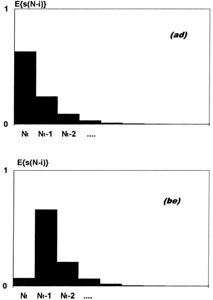
Fig. 6 illustrates the long-run average efficiency distribution of capital stocks for the case (ad) where technology is disembodied and every firm can strike an innovation and the case (be) where technology is embodied and only the best technology firms can strike an innovation. Since the shape of the efficiency distribution for the case (ae) where technology is embodied and every firm can strike an innovation is qualitatively the same as that of the case (ad), it is not shown here. The first graph has monotonically declining distributions with the declining rates initially slower than but later faster than that of geometric distribution. The second graph has a distribution which peaks at the second-best technology and then declines at the rate initially slower but later faster than that of geometric distribution.
In Section 2 we have seen that our Schumpeterian industry will never approach a classical or neoclassical equilibrium of uniform technology even in the long-run. If it will approach anything over a long passage of time, it is an equilibrium of disequilibria which reproduces a relative dispersion of efficiencies among firms in a statistically balanced form. We have now seen that even the persistent pressure of Darwinian selection mechanism is incapable of restoring classical or neoclassical equilibrium in the long-run state of our Schumpeterian industry. The process of capital accumulation will interact with the processes of innovation and imitation at the micro-level of firms only to maintain, at best, the relative configuration of its state of technology in a statistically balanced form.
3.4. Pseudo-aggregate production functions
Fig. 6. Long-run average distribution of capital stocks, (ad) when technology is disembodied and every firm can innovate, and (be) when technology is embodied and only the best technology firms can innovate.
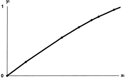
Fig. 7. A “pseudo-aggregate” production function.
of demand. Because of the fixed proportion technology (10), we can represent the level of employment associated with this output asLt =e−λNtYt. When the demand reaches the total capacity of the best technology bkt(Nt)=st(Nt)bKt, a further increase in demand is absorbed solely by an increase in price, while output is kept at the capacity level. But when the price reaches the wage cost of the second-best technology or whenPt =Wte−λ(Nt−1), the second-best capital stocks start to join the production and all the increase in demand is absorbed by a corresponding increase in output. Then, the relation between Yt and Lt can be given byLt =e−λNtst(Nt)bKt+e−λ(Nt−1)(Yt −st(Nt)bKt)until Ytreaches the total productive capacity of the first- and second-best technology(st(Nt)+st(Nt −1))bKt. In general, when(st(Nt)+ · · · +st(Nt−i))bKt ≤Yt < (st(Nt)+ · · · +st(Nt−i−1))bKt, the relation between Yt and Ltcan be given by
Lt =(st(Nt)+ · · · +eλist(Nt−i)+eλ(i+1)(Yt/bKt −(st(Nt) + · · · +st(Nt −i)))bKte−λNt.
If we divide this relation by bKte−λNt, we can express the efficiency labor–capacity ratio
xt ≡eλNtLt/bKt as a function of the output–capacity ratioyt ≡Yt/bKt as
xt =st(Nt)+ · · · +eλist(Nt −i)+eλ(i+1)(yt−(st(Nt)+ · · · +st(Nt−i))), where st(Nt)+ · · · +st(Nt−i)≤yt < st(Nt)+ · · · +st(Nt −i−1). (23) Fig. 7 depicts the inverse of the above relation in a Cartesian diagram which measures efficiency labor–capacity ratio xt along the horizontal axis and output–capacity ratio yt along the vertical axis. It is not hard to see that this relation satisfies all the properties a neoclassical production function is supposed to satisfy.10 Ytis linearly homogeneous in Lt and Ktbecauseyt ≡Yt/bKtis a function only ofxt ≡eλNt Lt/bKt. Though not smooth, this relation also allows a substitution between Kt and Ltand satisfies the marginal productivity principle:∂−yt/∂xt ≤1/Pt =e−λNt Wt/pt (=efficiency real wage rate)≤∂+yt/∂xt. (Here,∂−y/∂x and∂+y/∂x represent left- and right-partial differentials, respectively.) Yet,
the important point is that this is not a production function in the proper sense of the word!
It is a mere theoretical construct summarizing the production structure of the industry as a whole, and has little to do with the actual technological conditions of the individual firms working in the industry. As a matter of fact, the technology each firm uses is a Leontief-type fixed proportion technology which does not allow any capital/labor substitution. It is in this sense that we call the relation (23) a ‘short-run pseudo-aggregate production function.’
The shape of this function is determined by the efficiency distribution of capital shares
{st(n)}. Hence, as this distribution changes, the shape of the pseudo-production function also changes, and in our Schumpeterian industry, the efficiency distribution of capital stocks is incessantly changing over time as a result of dynamic interplay among innovations, imi-tations and capital growth. The most conspicuous feature of the short-run pseudo-aggregate production function is therefore its instability.
In the long-run, however, we know we can detect a certain statistical regularity in the rela-tive form of capital share distribution out of its seemingly unpredictable movement. We can thus expect to detect a certain statistical regularity in the relative form of pseudo-aggregate production function out of its seemingly unpredictable movement as well.
To see this, let us first note that by (23),xt = eλ0st(Nt)+ · · · +eλist(Nt −i)when
yt =st(Nt)+ · · · +st(Nt−i). Taking expectation, we then have
E(xt)=E{st(Nt)+ · · · +eλist(Nt−i)} when
E(yt)=E{st(Nt)+ · · · +st(Nt−i)}. (24)
Thus, under Hypotheses (IN-a) and (CG-d), if we lett → ∞, we have by (21ad),
E(xt)→(1−Γζ)(1+eλ1Γ1+ · · · +eλiΓi) (25ad)
when
E(yt)→1−Γζ for i=0,
E(yt)→(1−Γζ)(iΓi +(i−1)Γ2+ · · · +Γi) for i=1,2, . . . , Nt −1, with an understanding thatE(xt)=0 whenE(yt)=0. Next, under Hypotheses (IN-a) and (CG-e), if we lett → ∞, we obtain by (21ae),
E(xt)→(1−Λζ)(1+eλ1Λ1+ · · · +eλiΛi) (25ae)
when
E(yt)→1−Λζ for i=0,
E(yt)→(1−Λζ)(iΛ1+(i−1)Λ2+ · · · +Λi) for i=1,2, . . . Nt−1, with an understanding thatE(xt)=0 whenE(yt)=0. Finally, under Hypotheses (IN-b) and (CG-e), if we lett→ ∞, we obtain by (21be),
E(xt)→1−Ωζ+(1−Ψζ)(eλ1Ω1+ · · · +eλiΨ1· · ·Ψi−1Ωi), (25be) when
E(yt)→1−Ωζ for i=0,
E(yt)→1−Ωζ+(1−ψζ)(Ω1+ψ1(Ω2+ · · · +ψi−1Ωi) . . .) for
with an understanding thatE(xt)= 0 whenE(yt) =0. If we span a convex hull of the points (E(xt), E(yt)) defined by each of the above long-run relations, respectively, we are able to generate the “long-run average pseudo-aggregate production functions” for the three versions of our evolutionary model.
Since the above three long-run average pseudo-aggregate production functions have vir-tually the same shape as that of the short-run pseudo-aggregate production function depicted in Fig. 7, we do not show them here in order to save space. What should be emphasized is that they all exhibit all the properties that neoclassical production functions should have! The long-run average output–capacity ratioE(yt)≡E(Yt/bKt)is indeed an increasing and con-cave function of the long-run average efficiency labor–capacityE(xt)≡E(eλNt Lt/Kt). Thus, it is as if the total work force Ltand total capital stock Ktwere jointly producing the total output Ytsubject to an aggregate neoclassical production function with Harrod-neutral (or pure labor augmenting) technological progress eλNt. It is as if we had entered the
Solo-vian world of neoclassical economic growth in which the growth process of the economy could be decomposed into the capital–labor substitution along an aggregate neoclassical production function due to capital accumulation and the constant outward shift of the ag-gregate neoclassical production function itself due to the manna-like technological progress. This is, however, a mere macroscopic illusion! If we zoomed the microscopic level of the in-dustry, the picture we would get is entirely different. What we would find out is the complex and dynamic interplay of many firms’ innovation, imitation and accumulation activities. It is just impossible to disentangle these microscopic forces and decompose the overall growth process into a movement along a well-defined aggregate production function and an out-ward shift of the function itself. As a matter of fact, the basic parameters,λ,µandν or
ξ, which determine the rate of pseudo-Harrod-neutral technical progress eλNt, are also the
parameters that determine the very shape of the pseudo-aggregate production function. (We already know from (7a) and (7b) that the long-run average rate of technological change is equal toλνF under Hypothesis (IN-a) andλF /P
i((1−1/F )i/(ξ+µi))under Hypothesis (IN-b).) We are after all living in a Schumpeterian world where the incessant reproduction of technological disequilibria prevents the pseudo-aggregate production function from col-lapsing into the fixed proportion technology of individual firms. It is, in other words, its non-neoclassical features that give rise to the illusion that the economy is behaving like a neoclassical growth model. Neoclassical growth accounting has no empirical content in our Schumpeterian world.
3.5. Concluding remarks
This paper has developed a series of simple evolutionary models that can be used to analyze the development of industry structure as a dynamic process moved by complex interactions among innovations, imitations and investments of satisficing firms striving for survival and growth. It has demonstrated that what the industry will approach over a long passage of time is at best a statistical equilibrium of technological disequilibria which maintains a relative dispersion of efficiencies in a statistically balanced form.
profits is a sign of economic disequilibria. Competition being perfect, the expansion of industry supply, the diffusion of technology and the entry of new firms will soon wipe out any profits in excess of interest payments and risk allowances. There should thus be no room for the theory of profits in the long-run description of the economy, once the interest rate and the risk premium are determined by the equilibrium conditions for intertemporal resource allocation under uncertainty. If, however, the state of technology will forever retain a feature of disequilibrium, the economy will keep generating positive profits no matter how long it is run. As Schumpeter (1950, p. 28) once remarked, “surplus values may be impossible in perfect equilibrium, but can be ever present because that equilibrium is never allowed to establish itself.” We have thus opened up a room for the long-run theory of profits. In fact, we already have all the theoretical apparatus for such a theory at hand, and all we have to do is to work it out in detail.11
The present paper has adopted the so-called ‘satisficing’ principle in its description of the firms’ behavior — firms do not optimize a well-defined objective function but simply follow fixed organizational routines in deciding their innovation, imitation and growth policies. Indeed, one of the purposes of this paper was to see how far we could go in our representation of the economy’s dynamic performance without relying on the traditional assumption of perfect rationality of business behavior, and it has even succeeded in ‘simulating’ all the macroscopic characteristics of neoclassical growth model, and yet, there is no denying that our strict evolutionary assumption of fixed organizational routines is as unrealistic as the neoclassical assumption of fully rational decision-making is. Where have all these organizational routines come from? How will they change over time? Another important agenda for the future research is to study the evolutionary process of these routines by injecting at least a modicum of rationality into our firms’ headquarters. This will not turn our evolutionary model into a neoclassical model. But it will, I hope, furnish us with a common ground with the recently emerged and rapidly growing literature on endogenous growth in neoclassical economics.12
Appendix A
The purpose of this appendix is to calculate the waiting period distributionW (t ) ≡ Pr{T (Nt+1)−T (Nt)≤t}. The probability that an innovation takes place during a time interval, [t, t+dt] for the first time since time 0 isW (t+dt )−W (t )=dW (t ). This is also the probability that no innovation has taken place during (0, t) and an innovation takes place during [t, t+dt]. Since the probability of the former equals 1−W (t )and that of the latter equalsνFdt under Hypothesis (IN-a) andξFft(Nt)dt under Hypothesis (IN-b), we get dW (t )=(1−W (t ))νFdtunder Hypothesis (IN-a), and dW (t )=(1−W (t ))ξFft(Nt)dt under Hypothesis (IN-b). They can be solved, respectively, as
11Indeed in Iwai (1998), I have already worked out such a theory for the simpler evolutionary model presented in Iwai (1984b).
W (t )=1−e−νFt for t≥0, (A.1a)
under Hypothesis (IN-a). This is (7a) of the text. It can also be calculated as
ω=
under Hypothesis (IN-b). This is (7b) of the text.
Appendix B
The purpose of this appendix is to deduce the long-run average efficiency shares of firms given by (9a) and (9b) in the main text.
The share of the best technology ft(Nt) emerges at T(Nt) and moves along (5) from that time onwards. Its value at t is thus determined by how far back T(Nt) was. Let Bt(z) denote “the backward waiting period distribution” defined byBt(z)≡Pr{s−T (Nt)≤z}. Then, a “renewal process”, the renewal theory tells us that Bt(z) will in the long-run approach a steady-state distributionR0z((1−W (s))/ω)dsindependent of t (see Feller (1966, p. 355)). Hence, under Hypothesis (IN-a), we obtain
E{ft(Nt)} →
This is the first line of (9a). Under Hypothesis (IN-b), we also obtain
E{ft(Nt)} →
This is the second line of (9a) in the main text. Next, under Hypothesis (IN-b), the innovator is always one of the former best technology users and discontinuous transition occurs only once and atT (Nt −i+1). Hence, we have
Substituting this as well as (B.2b) into (B.5b), we obtain
E{ft(Nt−i)} →
can be transformed into another first-order ordinary differential equation:y(t )′=(γ λζ+
in the case of an embodied innovation, we obtain (19e). As for (18d) and (18e), since they themselves are both linear first-order ordinary differential equations ofst(Nt−i), they can be easily solved to obtain (20d) and (20e).
Appendix D
The purpose of this appendix is to deduce (21ad), (21ae) and (21be). We have to deal with each of them separately.
(ad). The case of Hypotheses (IN-a) and (CG-d). The capital share of the best technol-ogy st(Nt) emerges at T(Nt) and moves along a curve (19d). LetΘ(z;sT (Nt)(Nt))define
Under the assumption of disembodied technology, an innovator can implement a new tech-nology into all of its capital stocks at the time of its success. This means that unlike the initial value of the firm sharefT (Nt)(Nt)which always equals 1/F, the initial value of the
capital sharesT (Nt)(Nt)varies, depending on the history of the innovator’s capital share.
Nonetheless, since under Hypothesis (IN-a) every firm has an equal chance for innovation, we also know that its expected value must be equal to the average capital share which is tautologically equal to 1/F. In this paper I will use this average capital share as an approx-imation ofsT (Nt)(Nt). (In the case where only the best technology firms can innovate, I
have not come up with a good approximation ofsT (Nt)(Nt), and this is the reason why I
have not been able to deduce any explicit formulae for the long-run average capital shares under Hypotheses (IN-b) and (CG-d).) Then, since dBt(z)=dW (z)=νFe−νFzdzunder Hypothesis (IN-a), (D.1d) is seen to be equal to 1−Γζ,whereΓiis defined by (22ad), as in the first line of (21ad).
st(Nt −i)=
Under Hypothesis (IN-a) the probability that the innovator belongs to one of the users of technologyNt −iis its very shareft(Nt −i)and the expected capital share of each member isst(Nt −i)/Fft(Nt −i), so that the expected reduction of its capital share at each innovation time,E{sT (Nt−m)(Nt −i)/sT (Nt−m−0)(Nt −i)}is equal to 1−1/F for m=i−1, i−2, . . . ,0. Again approximatingsT (Nt−m)(Nt−m)by 1/F, we can express the
expected value of the first, the second, etc., the penultimate and the last term of the RHS of (D.2d), respectively, as
Γιis defined by (22ad). Hence, we obtain the second line of (21ad).
(ae). The case where Hypotheses (IN-a) and (CG-e) hold. In the case of embodied tech-nological change, the capital share of the best technology st(Nt) emerges with a mass of
Since dBt(z)→νFe−νFdzast→ ∞under Hypothesis (IN-a), this expression converges to the first line of (21ae). Next, since (20e) is identical with (20d) with sT (Nt)(Nt) = σ/(1+σ ), the capital shares of the lesser technologiesst(Nt −i)can also be expressed by (D.2d). Under hypothesis (CG-e) an innovation creates a new capital share of the best technology equal toσ/(1+σ )and is expected to reduce all the capital shares of the lesser technologies uniformly by the factor ofσ/(1+σ ). Hence, the expected value of the terms
(1/(1−sT (Nt−i+1)(Nt −i+1)))(sT (Nt−i+1)(Nt−i)/sT (Nt−i+1−0)(Nt−i))becomes all
equal to 1, and the expected value of the first, the second, etc., the penultimate and the last line of the RHS of (D.2d), respectively, becomes equal to
Z t−T (Nt)
0
(1−Π (z))e−γ λ(i−ζ )zdBt(z),
Z t−T (Nt−1)
0
(1−Π (z))exp{−γ λ(i−1−ζ )z}dW (z), . . . ,
Z t−T (Nt−i−1)
0
(1−Π (z))e−γ λ(1−ζ )zdW (z),
Z t−T (Nt−i)
0
Π (z)dW (z).
Noting that dW (z)=νFe−νFdzand dBt(z)→νFe−νFdzunder Hypothesis (IN-a), these expressions converge toΛi, Λi−1, . . . , Λ1and 1−Λζ ast → ∞, whereΛi is defined by (22ae). This leads to the second line of (21ae).
(be). The case where Hypotheses (IN-b) and (CG-e) hold. All the formulae for this case is identical with the previous case, except thatW (z) = 1−((1−ϕ(z))/(1−1/F ))ξ /µ
and dBt(z)→(1−W (z))dz/ω. Hence,E{st(Nt)} →1−Ωζ and this is the first line of (21be). Also the expected value of the first, the second, etc., the penultimate and the last line of the RHS of (D.5), respectively, converge toΩiΨi−1, . . . , Ψ1and 1−Ψζ, whereΩi andΨi are defined by (22be) and (22be′). We can then obtain the second line of (21be).
References
Aghion, P., Howitt, P., 1992. A model of growth through creative destruction. Econometrica 60 (2).
Aghion, P., Howitt, P., 1997. A Schumpeterian perspective on growth and competition, in: Kreps, D., Wallis, K. (Eds.), Advances in Economics and Econometrics: Theory and Applications, Proceedings of the Seventh World Congress, Vol. II. Cambridge University Press, Cambridge (Chapter 8).
Anderson, E.S., 1994. Evolutionary Economics: Post-Schumpeterian Contributions. Pinter, London.
Arrow, K.J., 1962. Economic welfare and the allocation of resources for inventions, in: Nelson, R.R. (Ed.), The Role and Direction of Inventive Activity. Princeton University Press, Princeton, NJ.
Barro, R., Sala-i-Martin, 1999. Economic Growth. MIT Press, Cambridge, MA.
Coleman, J.E., Katz, E., Menzel, H., 1957. A diffusion of an innovation among physicians. Sociometry 24 (1). Cox, D.R., Miller, H.D., 1965. The Theory of Stochastic Process. Wiley, New York.
Dossi, G., Freeman, G., Nelson, R., Silverberg, G., Soete, L. (Eds.), 1988. Technical Change and Economic Theory. Pinter, London.
Feller, W.W., 1966. An Introduction to Probability Theory and its Applications. Wiley, New York.
Franke, R., 1998. Wave trains and long waves: a reconsideration of Professor Iwai’s Schumpeterian dynamics, in: Dell Gatti, D., Gallegati, M., Kirman, A. (Eds.), Market Structure, Aggregation and Heterogeneity. Cambridge University Press, Cambridge.
Iwai, K., 1984a. Schumpeterian dynamics: an evolutionary model of innovation and imitation. Journal of Economic Behavior and Organization 5 (2).
Iwai, K., 1984b. Schumpeterian dynamics, Part II: Technological progress, firm growth and ‘economic selection’. Journal of Economic Behavior and Organization 5 (3).
Iwai, K., 1998. Schumpeterian dynamics: a disequilibrium theory of long-run profits (CIRJE discussion paper series F-30, Faculty of Economics, University of Tokyo, December 1998). In: Punzo, L. (Ed.), Cycle, Growth and Structural Change. Routledge, London.
Iwai, K., 1999. Persons, things and corporations: corporate personality controversy and comparative corporate governance. American Journal of Comparative Law 47 (4).
Metcalfe, J.S., Saviotti, P. (Eds.), 1991. Evolutionary Theories of Economics and Technological Changes. Harwood, Reading, MA.
Nelson, R., Winter, S., 1982. An Evolutionary Theory of Economic Change. Harvard University Press, Cambridge, MA.
Romer, P.M., 1990. Endogenous technological change. Journal of Political Economy 98 (1). Sato, K., 1975. Production Functions and Aggregation. North-Holland, Amsterdam. Schumpeter, J.A., 1939. Business Cycles. McGraw-Hill, New York.
Schumpeter, J.A., 1950. Capitalism, Socialism and Democracy, 3rd Edition. Rand McNally, New York. Schumpeter, J.A., 1961. The Theory of Economic Development. Oxford University Press, Oxford. Segerstrom, P.S., 1991. Innovation, imitation and economic growth. Journal of Political Economy 99. Simon, H.A., 1957. Models of Man. Wiley, New York.
Solow, R.M., 1957. Technical change and the aggregate production function, Review of Economics and Statistics. 39.