KEY WORDS:StreetGen, Street Modeling, RDBMS, Road Network, GIS database, kinetic hypothesys, Variable Buffer
ABSTRACT:
Streets are large, diverse, and used for conflicting transport modalities as well as social and cultural activities. Proper planning is essential and requires data. Manually fabricating data that represent streets (street reconstruction) is error-prone and time consuming. Automatising street reconstruction is a challenge because of the diversity, size, and scale of the details (∼cmfor cornerstone) required. The state-of-the-art focuses on roads and is strongly oriented by each application (simulation, visualisation, planning). We propose a unified framework that works on real Geographic Information System (GIS) data and uses a strong, yet simple hypothesis when possible to produce coherent street modelling at the city scale or street scale. Because it is updated only locally in subsequent computing, the result can be improved by adapting input data and the parameters of the model. We reconstruct the entire Paris streets in a few minutes and show how the results can be edited simultaneously by several concurrent users.
1. INTRODUCTION
Streets are complex and serve many type of purposes, including practical (walking, shopping, etc.), social (meeting, etc.), and cultural (art, public events, etc.). Managing existing streets and planning new ones necessitates data, as planning typically occurs on an entire neighbourhood scale. These data can be fabricated manually (cadastral data, for instance, usually are). Unfortunately, doing so requires immense resources in time and people.
Indeed, a medium sized city may have hundreds of kilometers of streets. Streets are not only spatially wide, they also are very plas-tic and change frequently. Furthermore, street data must be precise because some of the structuring elements, like cornerstones (they separate sidewalks from roadways) are only a few centimetres in height. Curved streets are also not adapted to the Manhattan hy-pothesis, which states that city are organised along three dominant orthogonal directions (Coughlan and Yuille, 1999).
The number and diversity of objects in streets is also particularly challenging. Because street data may be used for very different purposes (planning, public works, and transport design), it should be accessible and extensible.
Traditionally, street reconstruction solutions are more road recon-struction and are also largely oriented by the subsequent use of the reconstructed data. For instance, when the use is traffic simu-lation (Wilkie et al., 2012,Nguyen et al., 2014,Yeh et al., 2015), the focus is on reconstructing the road axis (sometime lanes), not necessarily the roadway surface. In this application, it is also essential that the reconstructed data is a network (with topological properties) because traffic simulation tools rely on it. However, the focus is clearly to reconstruct road and not streets. Streets are much more complex objects than roads, as they express the complexity of a city, and contains urban objects, places, temporary structures (like a marketplace). The precision of the reconstruction is, at best, around a metre in terms of accuracy.
Another application is road construction for the virtual worlds or driving simulations. In this case, we may simply want to create realistic looking roads. For this, it is possible to use real-life civil engineering rules, for instance using a clothoid as the main curve in highway (McCrae and Singh, 2009a,Wang et al., 2014). When
trying to produce a virtual world, the constructed road must blend well into its environment. For instance, the road should pass on a bridge when surrounded by water. We can also imitate real-world road-building constraints, and chose a path for the road that will minimise costs (Galin et al., 2010). Roads can even be created to form a hierarchical network (Galin et al., 2011). Reconstructed roads are nice looking and blend well into the terrain, but they do not match reality. That is, they only exist in the virtual world.
The aim may also be to create a road network as the base layout of a city. Indeed, stemming from the seminal work of (Parish and Muller, 2001), a whole family of methods first creates a road network procedurally, then creates parcels and extrudes these to create a virtual city. These methods are very powerful and ex-pressive, but they may be difficult to control (that is, to adapt the method to get the desired result). Other works focus on con-trol method (Chen et al., 2008,Lipp et al., 2011,Beneˇs et al., 2014). Those methods suffer from the same drawback; they are not directly adapted to model reality.
More generally, given procedural generation methods, finding the parameters so that the generated model will match the desired result is still an on-going research (inverse procedural modelling, like in (Martinovic and Van Gool, 2013) for fac¸ade, for instance). We start from rough GIS data (Paris road axis); thus, our modelling is based on a real road network. Then, we use a basic hypothesis and a simple road model to generate more detailed data. At this point, we generate street data for a large city (Paris); the result is one street network model. We use a widespread street network model, where the skeleton is formed by street axis and intersection forming a network. Then other constituents (lane, pedestrian cross-ing, markings, etc.) are linked to this network. We base all our work on a Relational DataBase Management System (RDBMS), to store inputs, results, topology, and processing methods.
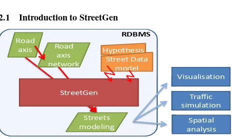
Figure 1: StreetGen in a glance. Given road axes, reconstruct network, find corner arcs, compute surfaces, add lanes and markings.
The design of StreetGen is a result of a compromise between theoretical and practical considerations. StreetGen amplifies data using a simple, yet strong hypothesis. As such, the approach is to attain correct results when the hypothesis appears correct and change the method to something more robust when the hypothesis appears wrong, so as to always have a best guess result.
Second, StreetGen has been designed to work independently at several different scales. It can generates street data at the city scale. The exact same method also generates street data interactively at the street scale.
Lastly, StreetGen results are used by different applications (visual-isation, traffic simulation, and spatial analysis). As such, the result is a coherent street data model with enforced constraints, and we also keep links with input data (traceability).
2.2 Introduction to RDBMS
We chose to use a RDBMS ((PostgreSQL, 2014) with (PostGIS, 2014)) at the heart of StreetGen for many reasons. First, RDBMSs are classical and widespread, which means that any application using our results can easily access it, whatever the Operating System (OS) or programming language. Second, RDBMSs are very versatile and, in one common framework, can regroup our input GIS data, a road network (with topology), the resulting model of streets, and even the methods to create it. Unlike file-based solutions, we put all the data in relation and enforce these relations. For instance, our model contains surfaces of streets that are associated with the corresponding street axis. If one axis is deleted, the corresponding surface is automatically deleted. We push this concept one step further, and link result tables with input tables, so that any change in input data automatically results in updating the result. Lastly, using RDBMS offers a multi OS, multi GIS (many clients possible), multi user capabilities, and has been proven to scale easily. We stress that the entirety of StreetGen is self contained into the RDBMS (input data, processing methods, and results).
2.3 StreetGen Design Principles
Input of StreetGen We use few input data, and accept that these are fuzzy and may contain errors.
The first input is a road axis network made of polylines with an estimated roadway width for each axis. We use the BDTopo1 product for Paris in our experiment, but this kind of data is avail-able in many countries. It can also be reconstructed from aerial images (Montoya-Zegarra et al., 2014), Lidar data (Poullis and You, 2010), or tracking data (GPS and/or cell phone) (Ahmed et al., 2014).
Using the road axis network, we reconstruct the topology of the network up to a tolerance using either GRASS GIS ((Neteler et al., 2012)) or directly using PostGIS Topology. We store and use the network with valid topology with PostGIS Topology. The second input is the roughly estimated average speed of each axis. We can simply derive it from road importance, or from road width (when a road is wide, it is more likely that the average speed will be higher).
The third input is our modelling of streets and the hypothesis we create.
Because the data we need can be reconstructed and there is a low requirement on data quality, our method could be used almost anywhere.
Street data model Real life streets are extremely complex and diverse; we do not aim at modelling all the possible streets in all their subtleties, but rather aim at modelling typical streets with a reasonable number of parameters.
First, we observe that street and urban objects are structured by the street axis. For instance, a pedestrian crossing is defined with respect to the street axis. At such, we centre our model on street axes.
Second, we observe that streets can be divided into two types : parts that are morphologically constant (same roadway width, same number of sidewalks, etc.), and transition parts (intersection, transition when the roadway width increases or decreases). We follow this division so that our street model is made of morpho-logically constant parts (section) and transition parts (intersection). The separation between transition and constant parts is the sec-tion limit and is expressed regarding the street axis in curvilinear abscissa.
Third, classical streets are adapted to traffic, which means that a typical vehicle can safely drive along the street at a given speed. This means that cornerstone in an intersection does not form sharp right turns that would be dangerous for vehicle tires. The most widespread cornerstone path in this case seems to be the arc of a circle, as it is the easiest form to build during public work. Therefore, we consider cornerstone path to be either a segment or
1
Figure 3: Street data model.
the arc of a circle. This choice is similar to (Wilkie et al., 2012) and is well adapted to the city, but not so well adapted to peri-urban roads, where the curve of choice is usually the clothoid (like in (McCrae and Singh, 2009b)), because it is actually the curve used to build highways and fast roads.
The surface of intersection is then defined by the farthest points on each axis where the border curve starts. In this base model, we add lanes, markings, etc.
Figure 4: 3 different radius size (3m, 4.9m, 7.6 m) for streets of various importancy, from real Paris data
Kinematic rule of thumb We propose basic hypotheses to at-tempt to estimate the radius of the corner in the intersection. We emphasise that these are rules of thumb that give a best guess result reasonably close to, and does not mean that the streets were actually made following these rules (which is false for Paris for instance).
Our first hypothesis is that streets were adapted so that vehicles can drive conveniently at a given speedsthat depends on the street type. For instance, vehicles tend to drive more slowly on narrow residential streets than on city fast lanes.
Our second hypothesis is that given a speed, a vehicle is limited in the turns it can make. Considering that the vehicle follows an arc of circle trajectory, a radius that is too small would produce a dangerous acceleration and would be uncomfortable. Therefore we are able to find the radiusrassociated with a driving speeds through an empirical functionf(s)−> r. This function is based on real observations of the French organisation SETRA (SETRA, 2006).
From our street data model and these kinematic rules of thumb, we deduce that if we roughly know the type of road, we may be able to roughly estimate the speed of the vehicles on it. From the speed, we can estimate a turning radius, which leads to the roadway geometry.
Schematically, we consider that a road border is defined by a vehicle driving along it at a given speed, while making comfortable turns.
2.4 Robust and Efficient Computing of Arcs
Goal The hypotheses in the above section allow us to guess a turning radius from the road type. This turning radius is used to re-construct the arcs of a circle that limits the junctions. The method must be robust because our hypotheses are just best guesses and are sometime completely wrong.
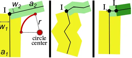
Given two road axis (a1, a2) that are each polylines, andnot segments), having each an approximate width (w1, w2) and an approximate turning radius (r=min(r1, r2), or other choosing rule), we want to find the centre of the arc of the circle that a driving vehicle would follow.
a
1a
2w
1w
2I
circle
center
r
I
I
1I
2Figure 5: Finding the circle centre problem. Left classical problem, middle and right using real-world data.
Method Our first method was based on explicit computing, as in (Wang et al., 2014), Figure 13. However, this method is not robust, and has special cases (flat angle, zero degree angle, one road entirely contained in another), is intricately two-dimensional (2D), and, most importantly, cannot be used on poly-lines. Yet real-world data is precisely made of polylines, due to data specification or errors.
Figure 6: The method to robustly find circle centres.
We are looking for the centre of the arc of the circle. Thus, by definition the centre could be all the places of distance ofd1 = w1+rfroma1and distance ofd2=w2+rfroma2.
We translate this into geometrical operations:
buf f eri, buffer ofaiwithdi
inter, the intersection of boundary of buffers, which is com-monly a set of point but can also be a set of points and curve. All those place could be circle centre.
closest, the point ofinterthat is the closest to the junction centre. We must filter this among the candidates in order to keep only the one that makes the most sense, given our hypotheses.
When hypothesis are wrong In some casesclosestmay be empty (when one road is geometrically contained in another con-sidering their width for instance). In this case our method fails with no damages, as no arc is created.
The radius may not be adapted to the local road network topology. This predominantly happens when the road axis is too short with respect to the proposed radius. In this case, we reduce the guessed radius to its maximal possible value by explicitly computing the maximum radius if possible.
It also happens that the hypotheses regarding the radius are wrong, which creates obviously misplaced arcs. We chose a very simple option to estimate whether an arc is misplaced or not and simply use a threshold on the distance between the arc and the centre of the intersection. In this case, we set the radius to a minimum that corresponds to the Paris lane separator stone radius (0.15m).
2.5 Computing Surfaces from Arc Centres
Border points Once the centre of circle is found, we can create the corresponding arc of circle by projecting the centre of the circle on both axis buffered bywi. In fact, we do not use a projection, as a projection on a polyline may be ill-defined (for instance projecting on the closest segment may not work). Instead, we take the closest point.
Similarly, we ’project’ the circle centre onto the road axis. We call these projection candidate border points. We have two or
Figure 7: Finding border points from arcs
less border points per axis per intersection. According to our intersection surface model, we only keep one of the candidates per axis per intersection, choosing the candidate that is the farthest from the intersection centre. We define the distance from the intersection centre by using the curvilinear abscissa, which is necessary because, in some odd cases, the Euclidian distance may be misleading.
I
border point border line
estimated normal
Figure 8: Creating the border line by cutting the section with local estimation of normal.
Section and intersection surface We compute the section sur-face by first creating border lines at the end of each section out of border points. The border lines are normal to a local straight approximation of the road axis. Then, we use these lines to cut the bufferised road axis to obtain the section surface.
At this point, it would be possible to construct the intersection surface by linking border lines to arcs, passing by the buffered road axis when necessary. We found it too difficult to do it robustly because some of the previous results may be missing or slightly false due to bad input data, wrong hypotheses or a computing precision issue.
We prefer a less specific method. We build all possible surfaces from the line set comprised of arcs, border lines, and buffered roads. We then keep only the surface that corresponds to the intersection.
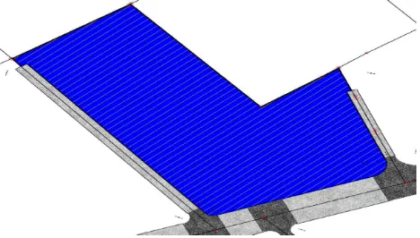
Variable buffer In the special case where the intersection is only a changing of roadway width, the arc of the circle transition is less realistic than a linear transition. We use a variable buffer to do this robustly. It also offers the advantage to being able to control the three most classical transitions (symmetric, left, and right) and the transition length using only the street axis.
Figure 9: Variable buffer for robust roadway width transition.
between vertices. One easy, but inefficient solution to compute it is to build circles and isosceles trapezoids and then union the surface of these primitives.
Lane, markings, street objects Based on the street section, we can build lanes and lane separation markings using a buffer. Note that simply translating the centre axis would not work with polylines.
Figure 10: Starting from center line (black), a translation would not create correct a lane (red). We must use the buffer (green).
Our input data contains an estimation of the lane number. Even when such data is missing, it can still be guessed from road width, road average speed, etc., using heuristics. The number of lane could also be retrieved from various remote sensing data. For instance, (Jin et al., 2009) propose to use aerial images. We can also build pedestrian crossings along the border lines. Using intersection surfaces, we build city blocks. We use the topology of the road network to obtain the surface of the face corresponding to the desired block. Then, we use Boolean operations to subtract the street and intersection surfaces from the face. This has the advantage that this still provides results when some of the street limiting the block have not been computed.
Figure 11: The blocks are generated even when some parts of the street network have not been computed.
2.6 Concurrency and scaling
One big query We emphasize that StreetGen is one big SQL query (using various PL/pgSQL and Python functions).
is not computingntimes one road surface. This is paramount because computing one road surface actually requires using its one-neighbours in the road network graph. Thus, computing each road individually duplicates a lot of work.
Third, we benefit from the PostgreSQL advanced query planner, which collects and uses statistics concerning all the tables. This means that the same query on a small or big part of the network will not be executed the same way. The query planner optimises the execution plan to estimate the most effective one. This, along with extensive use of indexes, is the key to making StreetGen work seamlessly on different scales.
One coherent streets model results One of the advantage of working with RDBMSs is the concurrency (the capacity for several users to work with the same data at the same time).
By default, this is true for StreetGen inputs (road network). Several users can simultaneously edit the road axis network with total guarantees on the integrity of the data.
However, we propose more, and exploit the RDBMS capacities so that StreetGen does not return a set of streets, but rather create or update the street modelling.
This means that we can use StreetGen on the entire Paris road axis network, and it will create a resulting streets modelling. Using StreetGen for the second time on only one road axis will simply update the parameters of the street model associated with this axis. Thus, we can guarantee at any time that the output street model is coherent and up to date.
Computing the street model for the first time corresponds to using the ‘insert’ SQL statement. When the street model has already been created, we use an ‘update’ SQL statement. In practice, we automatically mix those two statements so that when computing a part of the input road axis network, existing street models are automatically updated and non existing ones are automatically inserted. The short name for this kind of logic (if the result does not exist yet, then insert, else update) is ‘upsert’.
This mechanism works flawlessly for one user but is subject to the race condition for several users. We illustrate this problem with this synthetic example. The global streets modelling is empty. User1 and User2 both compute the street modelsicorresponding to a road axisri. Now, both users upsert their results into the street table. The race condition creates an error (the same result is inserted twice).
We can solve this race problem with two strategies. The first strategy is that when the upsert fails, we retry it until the upsert is successful. This strategy offers no theoretical guarantee, even if, in practice, it works well. We choose a second strategy, which is based on semaphore, and works by avoiding computing streets that are already being computed.
User1 result User2
table s_i exists?
no insert s_i
empty
s_i s_i exists?
update s_i
yes
User1 result User2
table s_i exists?
no insert s_i
empty
s_i
s_i exists?
insert s_i
no
error,
s_i
already exists
Figure 12: Left, a classical upsert. Right, race condition produces an error.
do nothing as long as those streets are already being computed by another StreetGen user. This strategy offers theoretically sound guarantees, but uses a lot of memory.
3. RESULTS 3.1 StreetGen
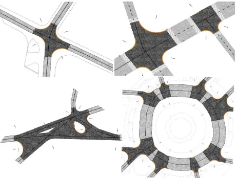
Robustness Overall, StreetGen generates the entire Paris road network. We started by generating a few streets, then a few blocks, then the sixth arrondissement of Paris, then a fourth of Paris, then the entire south of Paris, then all of Paris. Each time we changed scale, we encountered new special cases and exceptions. Each time we had to robustify StreetGen. We think it is a good illustration of the complexity of some real-life streets and also of possible errors in input data.
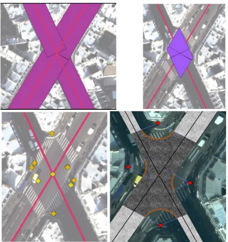
Quality Overall, most of the Paris streets seem to be adapted to our street data model. StreetGen results looks primarily realistic, even in very complex intersections, or overlapping intersections.
Figure 13: Example of results of increasingly complex intersec-tion.
Results are un-realistic in a few borderline cases, either because of the hypotheses or the limitations of the method. Those case are, however, easily detected and could be solved individually. Failure 1 is caused by the fact that axis 1 and 2 form a loop. Thus, in some special cases, the whole block is considered an intersection. This is rare and easy to detect. Failure 2 is caused by our method of computing intersection surface. It could be dealt with using the variable buffer. Failure 3 is more subtle and is because one axis is too short with respect to the radius. It could be fixed by taking
1 2
Figure 14: Various cases of failure from more severe to less severe (1 , 2 , 3). 1 : loop, 2 : bad buffer use, 3 : radius too big for network.
into consideration the next axis with roughly the same direction, but it would introduce special cases.
We compared the result of StreetGen with the actual roadways of Paris, which are available through Open Data Paris2. It clearly shows the limit of the input data, chiefly in roadway width estima-tions. Using interactive tools, it is possible to update the input
Figure 15: The estimated parameters may be far from reality (Left). It is, however, possible to manually or automatically fit the street model.
data so that it is closer to the reality, until a very good match is reached.
Scaling The entire Paris street network is generated in less than 10 minutes (1 core). Using the exact same method, a single street (and its one-neighbour) is generated in∼200ms, thus is lower than the human interactive limit of∼300ms.
SQL set operations We illustrate the specificity of SQL (work-ing on set) by test(work-ing two scenarios. In the first scenario (no-set), we use StreetGen on the Paris road axis one-by-one, which would take more than2hoursto complete. In the second scenario (set), we use StreetGen on all the axis at once, which takes about 10minutes.
Concurrency We test StreetGen with two users simultaneously computing two road axis sets sharing between 100% and 0% of road axis. The race condition is effectively fixed, and we get the expected result.
Parallelism We divided the Paris road axis network into eight clusters using the K-means algorithm3on the road axis centroid. This happens within the database in a few seconds. Then K users use StreetGen to compute one cluster (parallelism), which reducez the overall computing time to about oneminute.
4. DISCUSSION
Street data model Our street data model is simple and repre-sents well the roadway, but would need to be detailed in some
2
http://opendata.paris.fr/page/home/ 3
Figure 16: Clustering road axis centroid with K-Means, K=20, (black segments are convex hull).
aspects.
First, parking places are very abundant and important in Paris street organisation, yet our model cannot specifically deal with these.
Lanes are not a priority at the moment, and cannot have different width nor type (bus lanes, bicycle lanes, etc.).
Our model is just the first step towards modelling streets. In par-ticular, we do not integrate any urban objects in it. We could easily extend our street data model to add street objects positioned regarding the distance to the roadway and a curvilinear abscissa along the street axis as well as oriented with respect to the street axis.
Kinetic hypothesis Overall, kinetic hypotheses provide realistic looking results, but are far from being true in an old city like Paris. Indeed, a great number of streets pre-date the invention of cars. We attempted to find a correlation between real-world corner radius (analysing OpenDataParis through Hough arc of circle detection) and the type of road or the road’s average speed (from a GPS database). We could not find a clear correlation, except for fast roads; On those roads, the average speed is higher, and they have been designed for vehicles following classical engeneering rules.
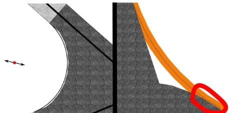
Precision issue All our geometrical operations (buffer, Boolean operations, distances, etc.) rely on PostGIS (thus GEOS4). We then face computing precision issues, especially when dealing with arcs. Arc is a data type that is not always supported, and thus it must be approximated by segments.
Figure 17: Example of a precision issue. Left, we approximate arcs with segments, which introduces errors. Right, the error was sufficient to incorrectly union the intersection surface.
StreetGen uses various strategies to try to work around these issues. However the only real solution would be to use an exact computation tool like CGAL (The CGAL Project, 2015). It would also allow us to compute the circle centres in 3D.
4
http://trac.osgeo.org/geos/
change the StreetGen results. Doing so ensures that any GIS software that can read and write PostGIS vector can be used as StreetGen GUI.
In some cases, we may have observations of street objects or sidewalks available, possibly automatically extracted from aerial images or Lidar, and thus imprecise and containing errors. We tested an optimisation algorithm that distorts the street model from best-guess StreetGen to better match these observations.
This subject is similar to Inverse Procedural Modeling, and we feel it offers many opportunities.
5. CONCLUSION
As a conclusion, we proposed a relatively simple street model based on a few hypotheses. This street data model seems to be adapted to a city as complex as Paris. We proposed various strategies to use this model robustly. We showed that the RDBMS offers interesting possibilities, in addition to storing data and facilities for concurrency. Our method StreetGen has ample room for improvements. We could use more sophisticated methods to predict the radius, better deal with special cases, and extend the data model to better use lane and add street objects. In our future work, we also would like to exploit the possibility of the interaction of StreetGen to perform massive collaborative editing. Such completed street modelling could be used as ground truth for the next step, which would be an automatic method based on detections of observations like sidewalks, markings, etc. Finding the optimal parameters would then involve performing Inverse Procedural Modelling.
6. ACKNOWLEDGEMENTS
The authors would like to thank reviewers for their suggestions, and colleagues for ideas and help, in particular G. Le Meur. This work was supported in part by an ANRT grant (20130042).
REFERENCES
Ahmed, M., Karagiorgou, S., Pfoser, D. and Wenk, C., 2014. A comparison and evaluation of map construction algorithms using vehicle tracking data. Geoinformatica 19(3), pp. 601–632.2
Beneˇs, J., Wilkie, A. and Kˇriv´anek, J., 2014. Procedural modelling of urban road networks. Computer Graphics Forum 33(6), pp. 132– 142.1
Chen, G., Esch, G., Wonka, P., M¨uller, P. and Zhang, E., 2008. Interactive procedural street modeling. ACM Trans. Graph. 27(3), pp. Article 103: 1–10.1
Galin, E., Peytavie, A., Gu´erin, E. and Beneˇs, B., 2011. Author-ing hierarchical road networks. In: Computer Graphics Forum, Vol. 30, pp. 2021–2030.1
Galin, E., Peytavie, A., Mar´echal, N. and Gu´erin, E., 2010. Proce-dural generation of roads. In: Computer Graphics Forum, Vol. 29, pp. 429–438.1
Jin, H., Feng, Y. and Li, Z., 2009. Extraction of road lanes from high-resolution stereo aerial imagery based on maximum likelihood segmentation and texture enhancement. In: Digital Image Computing: Techniques and Applications, 2009., IEEE, Melbourne, pp. 271–276.5
Lipp, M., Scherzer, D., Wonka, P. and Wimmer, M., 2011. Inter-active modeling of city layouts using layers of procedural content. In: Computer Graphics Forum, Vol. 30, pp. 345–354.1
Martinovic, A. and Van Gool, L., 2013. Bayesian grammar learn-ing for inverse procedural modellearn-ing. In: CVPR, 2013, IEEE, pp. 201–208.1
McCrae, J. and Singh, K., 2009a. Sketch-based path design. In: Proceedings of the Graphics Interface 2009 Conference, Cana-dian Information Processing Society, Kelowna, British Columbia, Canada, pp. 95 – 102.1
McCrae, J. and Singh, K., 2009b. Sketching piecewise clothoid curves. Comput. Graph. 33(4), pp. 452–461.3
Montoya-Zegarra, J. A., Wegner, J. D., Ladicky, L. and Schindler, K., 2014. Mind the gap: modeling local and global context in (road) networks. In: German Conference on Pattern Recognition (GCPR), p. 212 to 223.2
Neteler, M., Bowman, M., Landa, M. and Metz, M., 2012. GRASS GIS: a multi-purpose open source GIS. Environ. Model. Softw. 31, pp. 124–130.2
Nguyen, H., Desbenoit, B. and Daniel, M., 2014. Realistic road path reconstruction from GIS data. Computer Graphics Forum 33(7), pp. 259–268.1
Parish, Y. I. H. and Muller, P., 2001. Procedural modeling of cities. In: Proceedings of the 28th annual conference on Computer graphics and interactive techniques, pp. 301–308.1
PostGIS, d. t., 2014. PostGIS.http://postgis.net/.2 PostgreSQL, d. t., 2014. PostgreSQL. http://www. postgresql.org/.2
Poullis, C. and You, S., 2010. Delineation and geometric modeling of road networks. ISPRS Journal of Photogrammetry and Remote Sensing 65(2), pp. 165–181.2
SETRA, 2006. comprendre les principaux parame-tres de conception geometrique des routes. http: //catalogue.setra.fr/documents/Cataloguesetra/ 0004/Dtrf-0004044/DT4044.pdf. 3
The CGAL Project, 2015. CGAL User and Reference Manual. 4.6 edn, CGAL Editorial Board.7
Wang, J., Lawson, G. and Shen, Y., 2014. Automatic high-fidelity 3d road network modeling based on 2d GIS data. Advances in Engineering Software 76, pp. 86–98.1,3
Wilkie, D., Sewall, J., Lin, M. C. and Lin, M. C., 2012. Transform-ing GIS data into functional road models for large-scale traffic simulation. IEEE Trans. Vis. Comput. Graph. 18(6), pp. 890–901. 1,3
Wu, J., 2011. Improving the writing of research papers: IMRAD and beyond. In: Landsc. Ecol., Vol. 26number 10, pp. 1345 – 1349.1