STUDY OF AUTOMATIC IMAGE RECTIFICATION AND REGISTRATION OF
SCANNED HISTORICAL AERIAL PHOTOGRAPHS
H. R. Chen a*, Y. H. Tseng b
a Dept. of Geomatics, National Cheng Kung University, 701 Tainan, Taiwan – [email protected] b Dept. of Geomatics, National Cheng Kung University, 701 Tainan, Taiwan - [email protected]
Commission VI, WG VI/4
KEY WORDS: Historical aerial photographs, Image matching, Alignment of images, Rectification, Registration.
ABSTRACT:
Historical aerial photographs directly provide good evidences of past times. The Research Center for Humanities and Social Sciences (RCHSS) of Taiwan Academia Sinica has collected and scanned numerous historical maps and aerial images of Taiwan and China. Some maps or images have been geo-referenced manually, but most of historical aerial images have not been registered since there are no GPS or IMU data for orientation assisting in the past. In our research, we developed an automatic process of matching historical aerial images by SIFT (Scale Invariant Feature Transform) for handling the great quantity of images by computer vision. SIFT is one of the most popular method of image feature extracting and matching. This algorithm extracts extreme values in scale space into invariant image features, which are robust to changing in rotation scale, noise, and illumination. We also use RANSAC (Random sample consensus) to remove outliers, and obtain good conjugated points between photographs. Finally, we manually add control points for registration through least square adjustment based on collinear equation. In the future, we can use image feature points of more photographs to build control image database. Every new image will be treated as query image. If feature points of query image match the features in database, it means that the query image probably is overlapped with control images. With the updating of database, more and more query image can be matched and aligned automatically. Other research about multi-time period environmental changes can be investigated with those geo-referenced temporal spatial data.
1. INTRODUCTION
1.1 Value of Historical Aerial Photograph
With development of camera and aerial technology, aerial photograph and remote sensing images play a vital role within the geographical environmental study. Historical photographs directly provide the evidence of geographical environment in the past with “bird’s-eye” view. Many kinds of image data have increased since past to now, so analysis of temporal environmental changes become available with multi-period aerial photographs. The Research Center for Humanities and Social Sciences (RCHSS) of Taiwan Academia Sinica conserves and digital scans numerous historical aerial photographs and films continuously. Some of them have been geo-referenced manually, but most portion of them have not been registered since they have no GPS or IMU data for orientation assisting in the past. So we can’t know where the photographs were taken, which means the great amount of image data is useless if without geo-referencing information. Although the amount of photographs is too numerous to be processed only by manpower and the original interior parameter of these historical images disappeared after digital scanning, the probability of digital image processing is still feasible. For example, extracting and matching features between different aerial images, or using dense image matching for automatic reconstruction of buildings can be finished with computer vision. In this research, we use computer vision of digital image processing to show the feasibility and efficiency of dealing with the large quantity of historical aerial photographs.
* Corresponding author
1.2 Image Features and Image Matching
to remove outliers. This algorithm can estimate parameters for supposed mathematical model from a set of observation by iteration, and remove outliers by threshold. After RNASAC, we can acquire many conjugated points of historical aerial photographs. And we generalized tie points from these conjugate points by automatic programing, these tie points can be used to network adjustment of photogrammetry. After extracting image features, we only have to deal with point data instead of image data. That is, less consumption of computer calculation and better efficiency.
1.3 Rectification and Registration
After image matching and generating tie points automatically, we manually add some control points for calculating parameters of coordinate transformation by network adjustment. In our research, every photograph can be rectification and registration by 2D affine transformation or 2D projective transformation. These two kinds of transformation are both suitable for flat area. We developed an efficient way for matching historical aerial photographs and generating tie points automatically, and we only need to manually add some control points from recent satellite image for the final network adjustment. Registration means that those historical aerial photographs have been geo-referencing into the ground coordinate, and rectification means resampling of photographs by the parameters of coordinate transformation. Those historical aerial photographs became spatiotemporal data after geo-referencing. These historical material become more useful for analysis of temporal environmental changes or some research about coastal, land use, and urban planning.
2. DATA
2.1 Historical Aerial Photographs
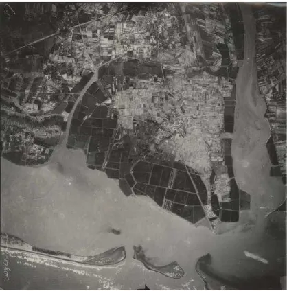
Historical aerial photographs provide the most direct and plentiful information about land cover from past to now, and they are the truest evidences for the analysis of temporal environmental changes. We can understand environmental change or natural landscape transformation by aerial photographs. The Research Center for Humanities and Social Sciences (RCHSS) of Academia Sinica which is the most preeminent academic institution of Taiwan conserves numerous historical maps and aerial photography films with coverage of Taiwan and mainland China. For preserving these valuable historical materials with another storage media, they successively scanned them into digital photographs. Although the interior parameters of the original photographs had disappeared after digital scanning, those digital historical aerial photographs became more convenient for processing of computer vision. Figure 1 shows one example of digital scanned historical aerial photograph, whose resolution is 15692 by 13217 pixels. And its GSD (ground sampling distance) is about 0.6 meters. The film was scanned with a Kodak colour control patches which represent the quality of colour. Due to the same pattern of the colour control patches, there will be some extra matching beyond the historical aerial image. It will directly influence the result of image matching, and consume the resources like CPU and memory. For reducing computer consumption and diminishing the errors of wrong matching owing to the colour control patches, those images had been cropped into approximately 7558 by 7958 pixels. We also reduce the size of digital image so that we can do more test within shorter time and prevent the waste of time for waiting calculation of computer. Figure 2 shows the edited image. We used this kind of edited photographs for image matching, resampling, registration and rectification in this research.
Figure 1. Example of scanned photograph.
Figure 2. Example of edited photograph.
2.2 Recent Satellite Image
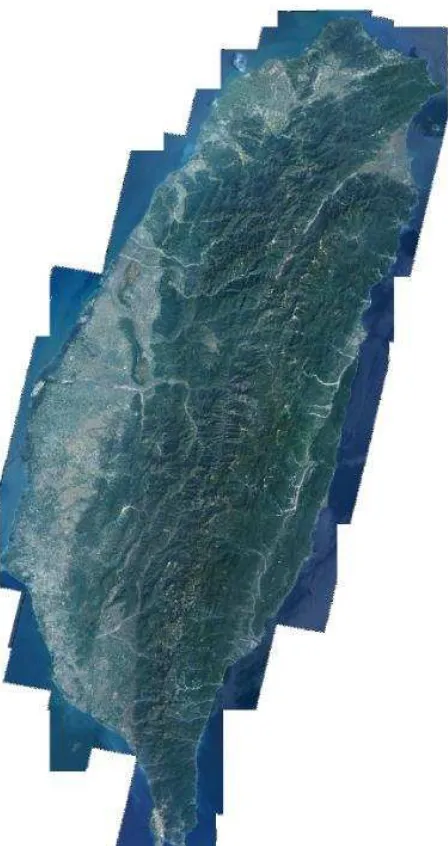
After laborious process that we found corresponding control points, we added them to the network adjustment with tie points which derived from historical aerial photographs by SIFT and RANSAC. Finally, for geo-referencing and assessment of accuracy, we choose the Projected Coordinate Systems, TWD97, which was suitable for use in Taiwan.
Figure 3. FORMOSAT-2 satellite image of Taiwan.
3. METHOD
The test image data set contain 12 photographs (2 flight lines) which were taken by US military in June 1956 and has 50% side over-lap and 60% forward over-lap. Because the historical aerial photographs are digital format, we can process them by computer vision directly. First, we used SIFT algorithm to extract image features from them and do image matching. Second, we developed a program for generalizing photogrammetric conjugate points as tie points for network adjustment. Third, we manually selected corresponding control points from historical aerial photographs and recent satellite image and added them to the network adjustment for calculate the parameters of 2D affine transformation or 2D projective transformation. There are more detailed descriptions in the following paragraph.
3.1 Pre-process of Historical Aerial photographs
As aforementioned, the original historical aerial photographs had been cropped and reduced for better calculation efficiency and diminishing the expected matching errors due to the Kodak colour control patches. We can make sure that the whole procedure of this research is feasible without the waiting for execution time.
3.2 Image Matching by SIFT
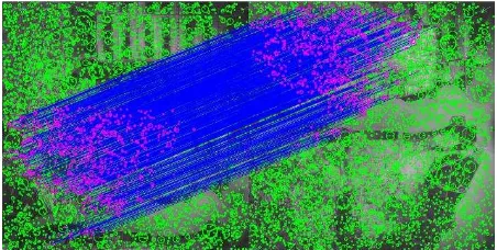
We used SIFT algorithm for extracting image features and matching image to automatically deal with the great amount of historical aerial photograph provided from RCHSS. Nowadays this algorithm is widely used in computer vision, and it has two advantages: great recognition for object and scene and high probability against a large database of features. Figure 4 shows an example of SIFT matching. The green circles represent the image features, and the blue lines connect the matched pairs whose feature descriptions are similar. There are some briefly introduction in the following paragraphs.
3.2.1 Scale-space extrema detection: First, SIFT algorithm transform the original image into scale-space by Gaussian window. The original image will be blur and blur with different scale of Gaussian window. Different scale means that this algorithm detects features in different resolution of image. Then every neighbouring images in the scale-space will be subtracted to each other in order to detect the local extrema value. It’s efficiency that use this concept of Difference of Gaussian (DoG) for calculating.
3.2.2 Feature localization: In this stage, SIFT algorithm use two kinds of threshold, peak threshold and edge threshold, to extract better features. Peak threshold filters the features whose peaks of the DoG scale space are too small. The edge threshold eliminates features whose curvature of the DoG scale space is too small for removing some points which are near edge.
3.2.3 Orientation assignment: Every SIFT feature has a major orientation (or more orientation) of gradient direction. It’s important to achieve the invariance to rotation.
3.2.4 Feature descriptor: Every feature point will be record as two kinds of descriptors. First one records the location of feature, direction of maximum gradient, and the scale of Gaussian scale-space. The second descriptor records every feature by 128-dimantion histogram for high distinctive. Then, by comparing the second descriptors between features, we can find some similar features of different images. In this research, we use these features to do image matching and generate tie points for network adjustment.
3.3 2D Coordinates Transformation
In this research, we use 2D affine transformation and 2D projective transformation for two purpose. In first purpose, SIFT and RANSAC, the transformations are used to compute the parameters of transformation from one image coordinate to another image coordinate. We compare the two kinds of transformations as the supposed transformation model in RANSAC. In the second purpose, we calculate the parameters of transformation from image coordinate to ground coordinate for registration of historical aerial photographs. Theoretically, 2D projective transformation will more fit than 2D affine transformation for both purpose in this research. For the first purpose, the normal vector of aerial images is not always point to the same direction, because the attitude of airplane always changes in the air. For the second purpose, the relation between image coordinate and ground coordinate will always change, because the same reason as mentioned above. There are more detailed descriptions about 2D affine transformation and 2D projective transformation as below.
3.3.1 2D Affine Transformation: This transformation preserves collinearity and contains six parameters which derived from scale, rotation, and offset of two directions. Equation (1) shows the expressed affine equation.
6
where (c, r) are image coordinate of historical aerial photograph, (E, N) are the corresponding TWD97 coordinate of FORMASAT-2 satellite image, and L1 - L6 are parameters of 2D affine transformation.
3.3.2 2D Projective Transformation: This transformation projects coordinate into another coordinate which’s axes are not parallel to original ones, so it has two more parameters than affine transformation. Historical aerial photographs were taken from airplane, and the orientation of view is impossible to be the same all the time. So this kind of transformation should be more suitable for historical aerial photographs than 2D affine transformation theoretically. Equation (2) shows the expressed transformation equation. The equation is nonlinear, so the calculate of solution needs initial values and iteration. And the former six parameters of 2D projective transformation is approximate with 2D affine transformation in the case of near-vertical aerial photographs, so we need to calculate the parameters of 2D affine transformation for the initial value of parameters of 2D projective transformation.
1 - L8 are parameters of 2D projective transformation.
3.4 Extract Better Conjugate Points by RANSAC
After SIFT image matching, there still are some similar image features which actually represent different points, so we use RANSAC algorithm to remove these wrong matchings. It’s an iterative method to estimate parameters of a supposed mathematical model from a set of observed data which contains
both inliers and outliers. In this research, we use two kinds of coordinate transformations as the supposed model and compare their performance. Figure 5 shows an example of SIFT matching after RANSAC. There are two major steps which repeat iteratively in RANSAC as below.
3.4.1 Randomly select subset and calculate supposed model: In this step, we have to suppose a mathematical model. In this research, we use 2D affine transformation and 2D projective transformation as the supposed model. Then randomly select observations as a test subset, and calculate the parameters of the supposed model by the subset. In this research, there are 6 or 8 parameters of two kinds of transformation, respectively.
3.4.2 Test all observations in the original set: Use the parameters which are calculated in the previous step to test all observations in the whole set. Then we assess the model by counting the quantity of observations which are inliers for the supposed model. There will be a threshold here for filtering outliers. Within the times of iteration, repeat this two steps to find parameters which contain the largest quantity of inliers. Finally, use the most fit parameters to test all observations. Here need the second threshold to eliminates outlier. In this research, we not only compare the two kinds of transformation as the supposed model in the process of RANSAC, but also combine both of them for comparison. There are three important issues of RANSAC: how many observations for randomly selecting, how many times of the iteration and what model should we suppose? In this research, the quantity of randomly selecting is about 20, the times of the iteration is 10000, and the supposed model are 2D affine transformation and 2D projective transformation. We will do more test about this issues in the future.
Figure 5. Example of removing outliers by RANSAC.
3.5 Matching Matrix of Recording result and Automatically Generate Tie Points
Photographs 1 2 3 4 5 6 7
1 64 4 3 68 3 1
2 639 80 161 53 0
3 1564 181 175 174
4 43 443 525
5 1150 170
6 183
7
Table 6. Example of matching record matrix.
3.6 Manually Select Control Points for Registration and Accuracy Assessment
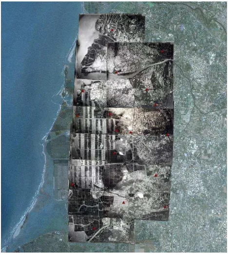
For registration of historical aerial photographs, we manually selected control points between historical aerial photographs (1956) and FORMOSAT-2 satellite images (2015). Figure 7 shows the same area of FORMOSAT-2 satellite images. These control points were added to network adjustment to calculate the parameters of 2D affine transformation or 2D projective transformation for coordinate transformation. This step is the most laborious, because the land cover had changed through decades and colour tones of the two kinds of images are different. And the resolutions of historical aerial photographs and FORMOSAT-2 satellite images are different, too. These reasons make us difficult to select corresponding points for control points. So we hardly try to find the changeless point, such as the corner of farm and roads. Finally, we assessed the accuracy of control point after network adjustment. And the result of transformation parameters represents the exterior parameters of every photograph. So registration and rectification of historical aerial images could be achieved.
Figure 7. Result of 2D projective transformation.
3.7 Rectification and Resampling of Historical Aerial Photographs
After network adjustment, we obtained all exterior parameters of all historical aerial photographs. That means we acquire all the relation between historical aerial photographs and
FORMOSAT-2 satellite images, and all these photographs could be projected to ground coordinate, TWD 97. Every new TIFF image file (Tag Image File Format) should accompany TFW file (TIFF World File) which record six parameters of affine transformation. But in the case of 2D projective transformation, there are totally eight parameters. In this case, we have to apply image resampling by the exterior parameters. Figure 8 and Figure 9 show the results of registration and rectification via two kinds of transformation. And the red triangles are control points. There are more analysis and assessment in the next paragraph.
Figure 8. Result of 2D affine transformation.
4. RESULT
4.1 Performance of RANSAC
RANSAC is widely used in computer vision and image processing, because it has good result for estimating a supposed model and removing outliers. In this research, we use RANSAC to remove the outliers of image matching. And we test two kinds of supposed model: 2D affine transformation and 2D projective transformation since the image data are aerial photographs and satellite images which are both near-vertical. Considering about the situation of taking photographs by airplane, we can expect that the result of 2D projective transformation will better than 2D affine transformation. But the time consumption of projective case will more than affine case, because the former one need iteration. Except the two kinds of transformation, we also apply both of them into the two steps of RANSAC. Figure 10 shows the image pairs of testing RANSAC. The lower area of left image and the upper area of the right image are overlapped. Figure 11 shows the result of SIFT image matching without RANSAC. There are totally 1596 matched pairs of this image pair. Most of them look correct, but there are some wrong matching pairs beyond the overlapped area. So we use RANSAC to eliminate outliers. We compared three cases of supposed model as mentioned previously, and Figure 12 – 14 show their results respectively. The pink circles represent matching pairs which are inliers after RANSAC. We set the same thresholds for the two steps in RANSAC. The first threshold is 9 pixels and the second threshold is 1 pixel. In both two steps, the parameters of supposed model will be calculated. And the conjugated points of one image will transform to the other image by the parameters. If the distance of the conjugate points which have been transformed and the corresponding matched point of another image is less than threshed, these matching pairs will be consider as right conjugate points. The reason why we set lager value for the first threshold is that we want remove the obvious outliers in the first step and preserve the outstanding conjugated points in the second step. Table 15 shows some comparison of these three cases. The matching distribution of Case 1 is similar to Case 3, and the precision of transformation of Case 3 is better than Case 1. We think the reason is that the projective transformation in the second step of RANSAC eliminate more outliers than the other case whose supposed model of second step is affine transformation. The execution time of Case 2 is more than the other two, because it need iteration for both steps in RANSAC. But the result of Case 2 which use projective transformation for both steps of RANSAC is not good as expected. We think the reason is that the calculated parameters of first step in RANSAC are not good. Because the program might select some outliers randomly, and the solution of projective transformation will be bad. Then the threshold, one-pixel, of second step eliminate more matching pairs due to the reason above. There is an important issue about the “random select” of RANSAC. Because the points of random selecting might contain some outliers, the solution of supposed model will be incorrect. If we set a small value of threshold in the first step, many correct conjugate points will be considered as outliers. In the second step, the small threshold which we set one-pixel make sure that the conjugate points between image pairs is probable the same points. Probability is also an important issue about RANSAC. If we set more times of iteration, it will be more possible that randomly select the good conjugated points. And the solution of supposed model will be better, too. In this research, we set 100000 times of iteration for testing the three kinds of supposed model.
Figure 10. Image pairs of testing RANSAC.
Figure 11. The result of SIFT matching.
Figure 12. RANSAC result of Case 1.
Figure 13. RANSAC result of Case 2.
RANSAC Case 1 Case 2 Case 3 1st stage
Threshold: 9 pixel
Affine Projective Affine
2nd stage
Threshold: 1 pixel
Affine Projective Projective
Quantity of Table 15. Example of matching matrix.
4.2 2D Affine Transformation and 2D Projective Transformation
We test these two transformation for two issue, image matching and network adjustment, in this research. For the first issue, combine these two transformation into RANSAC will perform well as mentioned earlier. For the second issue, Figure 8 and Figure 9 show the result of registration after network adjustment by 2D affine transformation and 2D projective transformation, respectively. We can compare them with Figure 7, both results look good. But both of them have discontinuity at some line features (border of farm, road or river) if we zoom in to observe. We thought that is because the distribution of control points (the red triangle) is not uniform, or because of the distortion of lens.
4.3 Accuracy Assessment of Network Adjustment
There totally 1357 tie points and 17 control points in this case. Both transformation can provide quite good vision results of registration after network adjustment. We can expect that the accuracy of 2D projective transformation will better than the accuracy of 2D affine transformation, and Table 16 also support the argument. The residuals of control points of 2D projective transformation are all smaller than the other transformation. But the execution time has extreme disparity between two transformations as Table 17 shows, because the calculation of 2D projective transformation needs iteration.
Control point
2D Affine 2D Projective E(m) N(m) E(m) N(m)
Table 16. The residual of control points of two kinds transformation.
Transformation 2D Affine 2D Projective Execution time 12 min 2 hrs, 40 min
Table 17. The execution time of two kinds of transformation.
5. CONCLUSIONS
5.1 The Performance of automatically Image Matching
Using SIFT to extract conjugate point is very efficient and automatic. But the matching points are too numerous to check that if they are conjugate points or not. So we use RANSAC to remove wrong matching, and test three cases for comparison. Precisions of transformation of three cases are all less than one pixel. The precision of transformation of combine two kinds of coordinate transformation is the best. Because some large outliers have been eliminated in the first step of RANSAC with 2D Affine transformation, and the better inliers have been preserve in the second step with 2D Projective transformation. But it need more time for iteration than the simplest case, 2D affine transformation. Finally, tie points for network adjustment can be generated automatically.
5.2 The Performance of Registration and Rectification
We can implement the calculation of network adjustment after automatically generating tie points by SIFT and RANSAC, and manually selecting control points. The registration accuracy of control point is about one meter for 2D projective transformation and it is better than 2D affine transformation which’s several meters. We think this accuracy is good enough for many applications about change analysis of large area. But the execution time of the former transformation is too long. If we use original resolution image or more images in the future, efficiency of computation will be an important issue.
We also finished the rectification of historical aerial photographs by the parameters derived from network adjustment. That is, not only modern aerial photographs but also historical ones can be displayed in the same coordinate. In this study, the efficiency of automatically matching image and generating tie points has been proved. So it’s possible that the numerous historical aerial photographs could be automatically geo-referencing via computer vision in the future. That will make many other research or application of multi-period aerial photographs be possible to achieve.
ACKNOWLEDGEMENTS
In Taiwan, the Ministry of Science and Technology give us financial support so that we can do more research about processing historical aerial photographs.
RCHSS spend a lot of time and manpower to conserve and scan historical maps and aerial photographs. They provide us great amount of historical materials. Give us the chance that we can make these data more useful and valuable. Some researches which are relative to historical aerial photographs could process image data by our method and result.
REFERENCES
Harris, C. and M. Stephens. 1988. A combined corner and edge detector. Alvey vision conference, Citeseer.
Kim, J. S., C. C. Miller and J. Bethel. 2010. Automated Georeferencing of Historic Aerial Photography. Journal of Terrestrial Observation 2(1): 6.
Lowe, D. G. 2004. Distinctive image features from scale-invariant keypoints. International Journal of Computer Vision 60(2): 91-110.
Martin A. Fischler and Robert C. Bolles (June 1981). "Random Sample Consensus: A Paradigm for Model Fitting with Applications to Image Analysis and Automated Cartography". Comm. of the ACM 24 (6): 381–395.
Mikolajczyk, K. and C. Schmid 2004. Scale & affine invariant interest point detectors. International Journal of Computer Vision 60(1): 63-86.