www.elsevier.nlrlocaterisprsjprs
Review Paper
State-of-the-art of elevation extraction from satellite SAR data
Thierry Toutin
), Laurence Gray
Canada Centre for Remote Sensing, 588 Booth Street, Ottawa, Canada K1A 0Y7
Received 11 May 1999; accepted 24 November 1999
Abstract
Relative or absolute elevation extraction from satellite radar data has been an active research topic for more than 20 years. Various investigations have been made on different methods depending on the predominant ‘‘fashion’’ and data availability, leading each time to new developments to improve the capability and the applicability of each method. The paper presents an update of the state-of-the-art of elevation extraction from satellite SAR data. The performance and
Ž .
limitations of four different methods clinometry, stereoscopy, interferometry and polarimetry are reviewed, as well as their applicability to different satellite SAR sensors. Their advantages and disadvantages and how they are addressed during the data processing are also analysed. Finally, concluding remarks look at the complementarity aspects of each method to make the best use of the existing and future radar data for elevation extraction. Crown Copyrightq2000 Published by Elsevier Science B.V. All rights reserved.
Keywords: DEM; satellite SAR; clinometry; shape-from-shading; stereoscopy; interferometry; polarimetry
1. Introduction
With the advent of instruments that produce im-ages from electromagnetic radiation beyond wave-lengths to which the human eye and cameras are responsive, human ‘‘ vision and perception’’ has been greatly extended. Remote sensing has evolved into an important supplement to ground observations and aerial images in the study of terrain features, such as
Ž .
ground elevation. Digital elevation models DEMs are currently one of the most important data used for geo-spatial analysis. Unfortunately, DEMs of suffi-cient point density are still not available for many parts of the Earth, and when available, they do not always have sufficient accuracy. Since a DEM
en-)Corresponding author.
Ž .
E-mail address: [email protected] Th. Toutin .
ables easy derivation of subsequent information for various applications, elevation modeling has become an important part of the international research and
Ž .
development R & D programs related to geo-spatial data.
Due to high spatial resolution of civilian satellite
Ž .
synthetic aperture radar SAR sensors since the
Ž .
1980s with the Shuttle Imaging Radar SIR , a large number of researchers around the world have investi-gated the elevation modeling and the production of DEMs. Recent discussions on different aspects of radar for radargrammetry and for cartography can be
Ž . Ž .
found in Leberl 1990 and Polidori 1997 , respec-tively. Furthermore, the recent research in computer vision to model human vision has led to the advent of new alternatives applied to satellite imagery.
Since the elevation extraction is an active R & D topic, the objective of the paper is to update the
0924-2716r00r$ - see front matter Crown Copyrightq2000 Published by Elsevier Science B.V. All rights reserved.
Ž .
Ž .
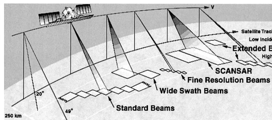
Fig. 1. Operating modes of RADARSAT-SAR C-band, HH polarisation .
previous reviews, mainly with the launch of the Canadian RADARSAT in 1995 and the research studies related to its different SAR imaging
capabili-Ž . Ž . Ž
ties Fig. 1 . Four different methods Fig. 2
clinom-.
etry, stereoscopy, interferometry and polarimetry to extract relative or absolute elevation are then re-viewed with their advantages and disadvantages. Their applicability to the different satellite SAR data is also presented. Finally, some concluding remarks on these methods and their complementarity, and prospects for the future with the next generation of satellites are drawn.
2. Clinometry
Shade, shadows and occluded areas are familiar phenomena that can help judge size and shape of objects by providing an impression of convexity and concavity. They are particularly helpful if the objects are very small or lack tonal contrast with their surroundings. These familiar phenomena are used to extract relative elevations of specific targets or ter-rain elevations from a single image. However, shad-owing and shading are sometimes confused.
2.1. Shadowroccluded areas
Ž
Shadow only provides localised cues along
spe-.
cial contours of shape, although the shadow of a
curved surface cast on another curved surface is very difficult to interpret. The shadow areas then occur when the ground surface is not illuminated by the source, while the occluded areas occur when the ground surface is not visible from the sensor.
Since the illumination source is the sensor with
Ž
monostatic i.e., transmit and receive antennas are
.
together SAR images, the effects of these two phe-nomena are mixed; shadow and occluded areas are then the same. Since the shadow areas are com-pletely without information, the boundaries of a cast shadow are then easier to determine than with visible
Ž .
and infrared VIR images. Depending on the SAR look-angles, only the steepest slopes can produce
Ž
shadowroccluded areas e.g., slopes larger than 678 and 518 for ERS-SAR and RADARSAT-F5,
respec-.
tively . The shadow and layover lengths can then be consistently measured only from vertical structures, such as buildings, towers, trees, etc. Consequently, the applicability of the method is reduced to very specific rugged terrain with strong cliffs. Relative heights can be derived from the cast shadow using simple trigonometric models and knowledge of the
Ž .
SAR geometry La Prade and Leonardo, 1969 . Since the shadow is shortened by the amount of layover due to vertical structures, the layover lengths have to be added to the shadow lengths in the computation. Using high-resolution simulated radar images, La
Ž .
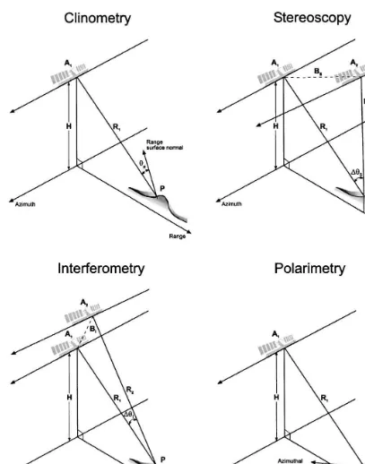
Fig. 2. Comparison of the geometry for the four elevation extraction methods: clinometry, stereoscopy, interferometry and polarimetry. Ai and H are the satellite position and altitude, respectively, R the slant-range component and h the elevation of a ground point P. For clinometry,u is the incidence angle in the plane defined by the range direction and the surface normal. For stereoscopy, Du is the
R S
Ž .
intersection angle, i.e., the difference between the two incidence angles and BS few hundred kilometres the baseline. For interferometry,
Ž . Ž .
Ž
of few man-made vertical structures buildings and bridge towers with 100–200 m elevation, e.g.,
Em-.
pire State building and Golden Gate bridge and hill
Ž .
peaks 50–150 m elevation with an average error of 1.5% and 2.4% of the elevation, respectively. Even though the elevation modeling is coarse, this corre-sponds to elevation accuracy of a few meters.
2.2. Shading
Shading is the variation of brightness exhibited in images. It arises primarily because some parts of a surface are oriented so as to reflect more of the
Ž
incident illumination towards the sensor Horn,
.
1975 . Since shading provides cues for the whole surface and not just along special contours, the sur-face slope and height can be estimated, given that the surface reflectivity function and the position of the
Ž .
illumination source are known see Fig. 2 top left . The application of the clinometry concept to SAR data is less evident due to the sensitivity of shading to reflective properties of the Earth’s surface. Radar-clinometry, as an adaptation of photoRadar-clinometry,
de-Ž .
veloped by Horn 1975 , has been further developed
Ž .
by Wildey 1984 regarding the mathematical
equa-Ž .
tions, and then again by Wildey 1986 regarding its operational feasibility in anticipation of the Magellan mission to map Venus. Radarclinometry capabilities and limitations are well known, even if the research
Ž
studies have been limited Frankot and Chellapa,
.
1988; Thomas et al., 1989, 1991; Guindon, 1990 . At first, the principle appears simple, essentially the inversion of a mathematical expression of the radar backscatter in terms of the albedo and the local incidence angle. The local slope is then computed from the pixel reflectivity value and transformed into relative elevation by integration pixel by pixel. In other words, shape-from-shading makes use of the sensitivity of the micro-topography, but it cannot provide absolute location. Some reference elevation information is needed to derive the absolute eleva-tion. Intrinsic radiometric and geometric ambiguities then limit the accuracy of this technique, when ap-plied to general terrain surfaces; the accuracy of derived slopes and elevation is generally of the order of few degrees and better than 100 m, respectively, depending on the image resolution and terrain relief.
Firstly, the SAR backscatter of the surface changes, if the surface properties vary from place to place and assuming uniform reflecting properties
Žconstant albedo , will recover a shape incidence. Ž .
angle that is different from the actual one. However, even with surfaces of varying reflectivity, a Lamber-tian model for homogeneous surfaces is often used for simplification. This approximation was first used
Ž .
with SAR by Wildey 1986 , and is now used in most research studies.
Ž
More sophisticated models Ulaby and Dobson,
.
1988 that take into account the SAR and surface
Ž
interaction surface geometry, vegetation, soil
prop-.
erties, geographic conditions, etc. have been devel-oped. They should now permit a more realistic
Ž
backscattering model of the intensity Paquerault and
.
Maıtre, 1997, 1998 than the traditional Lambertian
ˆ
model used for homogeneous surfaces. No attempt to extensively use these new models has been made, due to a relative decline of the interest of the scien-tific community in clinometry during the last 10 years. Other radiometric problems, which are not completely controlled and fully resolved, are specific
Ž .
to SAR sensors Guindon, 1990; Polidori, 1997 , namely speckle and miscalibration.
Secondly, the geometric ambiguity is related to the definition of the incidence angle. Even if it is accurately determined, it does not define uniquely the orientation of the surface but a set of possible orientations. Their normal directions describe a cone with the axis being the illumination direction. Since there are two degrees of freedom for the surface orientation, two angles to specify the direction of a unit vector perpendicular to the surface are needed
ŽHorn, 1975 . At each pixel, one brightness measure-.
ment gives only one equation for two unknowns. Additional constraints or assumptions have to be made to resolve this conic ambiguity. One
assump-Ž .
tion implemented by Wildey 1986 is the hypothesis of local cylindricity. It enforces a local continuity between adjacent pixels to define a local cylinder. Since there is no iteration in the solution process, the local cylindricity method is sensitive to integration approximations due to miscalibration and image noise. It then tends to accumulate these effects along the full DEM reconstruction leading to ‘‘pseudo
Ž . Ž .
SEASAT-Ž
SAR image over a high relief terrain 1200 m
eleva-.
tion range with 10–158 mean slopes . It was shown that the speckle caused large random errors in the order of hundreds of metres and miscalibration, a systematic bias in the order of tens of metres.
Other assumptions or constraints to resolve the conic ambiguity implemented by Frankot and
Chel-Ž .
lapa 1988 are the notions of integrability and regu-larisation. The first one states that heights can be integrated along any path, since these values are independent of the integration path. This constraint acts as a smoothing process and can reduce the slope errors by a ratio of 4 to 5. The second constraint limits the amount of allowable oscillation in the computed terrain surface, but does not significantly improve the results, perhaps indicating that most of the smoothing is coming from the integrability con-straint. Furthermore, they used an iterative approach starting from a coarse existing DEM. Differences between the grey values of the real image and the SAR synthetic image, predicted from the latest esti-mated DEM, are used to improve the terrain slopes and heights and to converge to the final DEM. As many as 300 iterations can increase the accuracy by
Ž .
a factor of 5 Leberl, 1990 . This approach mainly adds details of the micro-topography to the DEM
ŽThomas et al., 1991 . In conjunction with the inte-.
grability and regularisation constraints, this approach tends to spread out the speckle noise errors instead of propagating them only along the range profiles,
Ž
leading to slope errors of 18 to 28 only tested with .
simulated images .
Ž .
Thomas et al. 1989 expanded this iterative ap-proach to multiple images. Stereoscopy is first used to derive a DEM as a starting point of the shape-from-shading process. Some spot heights derived from stereoscopy or other sources can also be added as supplementary constraints of the estimated heights. Use of multi-image algorithms enables better stabil-ity and robustness with noisy images during the iteration procedure, as well as 5 to 10 times faster
Ž
convergence. Using two X-band SAR images 6-m
.
resolution, 7 looks acquired by the STAR-2 system of Intera Technologies, Canada, over a medium
re-Ž .
lief terrain 500-m elevation range , Thomas et al.
Ž1991 refined the radargrammetric DEM with this.
iterative two-image approach. As expected, the final DEM was not significantly more accurate than the
Ž .
radargrammetric DEM 22 m vs. 25 m , but the refinement of the details in the micro-topography was evident. However, all these constraints and re-fined processing algorithms do not fully resolve the two basic ambiguities.
Ž .
For the conic ambiguity, Guindon 1990 quanti-tatively demonstrated that the SAR image grey level is not an effective indicator of local incidence angle, and hence, is not an accurate measure of the overall local terrain surface normal direction. It is only a strong indicator of the range component of the ter-rain slope. It can therefore be used only to derive elevation profiles for individual range image lines. Consequently, using a single SEASAT-SAR image over a high relief area, he only evaluated the eleva-tion accuracy along range profiles, and obtained a slope and elevation accuracy of about 28to 38and 50 to 80 m, respectively.
Since no significant detectable information is available about azimuthal slope, an additional source of ‘‘azimuthal control’’ data is required to tie the adjacent range line elevation profiles to a common and absolute origin. Thus, Paquerault and Maıtre
ˆ
Ž1997. developed a two-step strategy to compute
these two components of the incidence angle. Firstly, they computed the range component from the backscatter pixel values, and integrated it along a range line. They then applied a contextual Marko-vian strategy to successively modify, in a random order, the slope orientation of each pixel in the
Ž .
image. This second step provided a way i to take into account the azimuth component of the incidence
Ž .
angle, ii to link together the adjacent range line
Ž .
elevation profiles, and iii to reduce the noise error propagation. The method seems to be more effective than the research studies previously described, since the extracted DEMs using a single-image technique have a consistent accuracy of about 30 m for various
Ž .
satellite data ERS, JERS, RADARSAT and
low-Ž
to-moderate relief terrain 200-m elevation range,
.
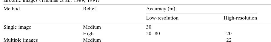
accu-Table 1
Ž . Ž
General results of shape-from-shading DEM accuracy. Low-resolution SAR around 30 m is for satellite images Guindon, 1990 with
. Ž .
SEASAT; Paquerault and Maıtre, 1997 with ERS, JERS, RADARSAT-Standard and high-resolution SAR less than 10 m for simulated orˆ
Ž .
airborne images Thomas et al., 1989, 1991
Ž .
Method Relief Accuracy m
Low-resolution High-resolution
Single image Medium 30
High 50–80 120
Multiple images Medium 22
High 80
racy varies regularly from 13 to 33 m, and from 258 to 458look-angles it varies from 25 to 32 m. Table 1 summarises the general results of elevation extrac-tion or DEM generaextrac-tion with the shape-from-shading method.
Despite the developments and the interesting re-sults in the mid 1990s, SAR shape-from-shading remains a marginal technique, applied mainly in difficult situations such as tropical land-cover or extraterrestrial sites without ground truth. It is mainly due to the fact that the radiometric ambiguity be-tween the terrain albedo, the radar backscattering cross-section and the incidence angle is rarely solved, except on a homogeneous terrain surface with a Lambertian model. However, Earth parts that are not or poorly mapped approximate to a large extent a homogeneous Lambertian surface.
3. Stereoscopy
Disparity and convergence are the two cues when viewing stereo imagery. Disparity predominates when viewing radar images, but the shade and shadow cues also have a strong and cumulative effect. For example, with a quasi-flat terrain, the shade and shadow cues overcome the disparity effect when
Ž
viewing pseudoscopically a radar stereo-pair Toutin
.
and Amaral, 2000 . Due to the specific geometric and radiometric aspects of SAR images, it may take our brain time to assimilate this unnatural stereo viewing, mainly when both geometric and
radiomet-Ž .
ric disparities are large Toutin, 1996 . However,
Ž
since depth perception is an active process brain and
.
eye and relies on an intimate relationship with object recognition, after training, radar images can
be viewed in stereo as easily as VIR satellite images. This disparity principle is used in radargrammetry to compute the terrain elevation from the measured
Ž
parallaxes between the two images see Fig. 2 top
.
right .
3.1. Application to SAR sensors
In the 1960s, stereoscopic methods were first applied to radar images to derive ground elevation
Ž
leading to the development of radargrammetry La
.
Prade, 1963 . He showed that some specific SAR stereo configurations would produce the same eleva-tion parallaxes as produced by aerial images. Conse-quently, elevation could be measured with traditional
Ž .
stereo-plotters. Furthermore, Carlson 1973 devel-oped a technique to generate radar stereo images acquired form one flight path with fore and aft squinted looks, which were easier to view and mea-sure than the traditional technique with two flight paths. However, the lack of radar stereo pairs led
Ž
mainly to theoretical studies Rosenfield, 1968;
Gra-.
cie et al., 1970; Leberl, 1979 or simulated data
Ž
processing experiments Kaupp et al., 1983; Domik,
.
1984 .
During the 1980s, improvements of SAR systems, with parallel investigations into their theory, have allowed the demonstration of stereo radar with same-side or opposite-side viewing. These
theoreti-Ž .
cal studies Leberl, 1979 and practical experiments
ŽFullerton et al., 1986; Toutin, 1996 confirm that.
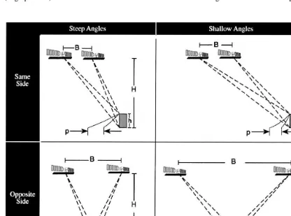
correspond-ing points and features more difficult. Fig. 3 illus-trates the intersection geometry with the radar
eleva-Ž
tion parallax for different stereo configurations same
.
vs. opposite side, steep vs. shallow look-angles . To obtain good geometry for stereo plotting, the
Ž .
intersection angle Fig. 3 should be large in order to increase the stereo exaggeration factor, or equiva-lently the observed parallax, which is used to deter-mine the terrain elevation. Conversely, to have good
Ž
stereo-viewing, the interpreters or the image
match-.
ing software prefer images as nearly identical as possible, implying a small intersection angle. Conse-quently, large geometric and radiometric disparities together hinder stereo-viewing and precise stereo plotting. Thus, a compromise has to be reached
Ž
between a better stereo-viewing small radiometric
.
differences and more accurate elevation
determina-Ž .
tion large parallax .
The common compromise for any type of relief is to use a same-side stereo-pair, thus, fulfilling both conditions above. Unfortunately, this does not max-imise the full potential of stereo radar for terrain relief extraction. Different compromises can then be realised to reduce either geometric or radiometric disparities. To reduce the radiometric differences of an opposite-side stereo-pair, the radiometry of one
Ž
image can be inverted Yoritomo, 1972; Fullerton et
. Ž .
al., 1986 . Fullerton et al. 1986 added a local brightness change to exclude some image features from the radiometric inversion. Another potential compromise is to use opposite-side stereo-pairs over
Ž .
rolling topography Toutin, 1996 . The rolling topog-raphy reduces the parallax difference and also the
Ž
radiometric disparities no layover and shadow, little
.
foreshortening making possible simultaneously good stereo-viewing and accurate stereo-plotting. A last
Ž . Ž .
approach to minimise the geometric disparities is to pre-process the images using a large grid spacing or low accuracy DEM, as it has been applied with success to iterative hierarchical SAR image matching
ŽSimard et al., 1986 ..
However, with spaceborne platforms, parallel
Ž .
flights from opposite or same side are very rare. Even sun-synchronous satellite orbits are parallel only near the Equator. Elsewhere, crossing orbits or convergent stereo configuration must be considered. If rigorous intersection geometry is applied, no dif-ferences exist between computations for parallel or-bits and those for crossing oror-bits. That has been confirmed with the SIR-ArB shuttle missions of
Ž
1981 and 1984 Kobrick et al., 1986; Leberl et al.,
.
1986a; Simard et al., 1986 . The first two studies processed radar images at an analytical stereo-plotter, the Kern DSR-1, adapted to process stereo SAR images. The last study used a fully digital method with iterative hierarchical matching. The results achieved for the DEM were on the order of 60 to 100 m mainly due to the poor SIR-A resolution, or radiometric and geometric image quality. Further-more, the SIR-B SAR was the first system for creat-ing and comparcreat-ing different stereo-pairs with ray
Ž
intersection angles ranging from 58to 238 Leberl et .
al., 1986b .
Ž
Since the launch of different satellite sensors
Al-.
maz, ERS, JERS, etc. in the beginning of the 1990s, radargrammetry again became a hot R & D topic. The Russian Almaz-1 SAR system acquired images with different angles to obtain stereo-images in the
lati-Ž .
tude range from 08 to 728. Yelizavetin 1993 digi-tally processed two images with 388and 598 look-an-gles over a mountainous area of Nevada, USA. No quantitative results were given. Stereoscopy with ERS-SAR data has been obtained using an image
Ž .
with its normal look-angle 238 and a second image
Ž . Ž .
with the Roll-Tilt Mode RTM angle 358 to
gener-Ž .
ate a same-side stereo-pair Raggam et al., 1993 . However, this ERS stereo configuration is very rare due to the limited amount of SAR data acquired in RTM. Another ERS stereo configuration can also be
Ž .
used with two normal look-angle 238 images from ascending and descending orbits to generate an
op-Ž .
posite-side stereo-pair Toutin, 1995, 1996 .
Com-Ž .
parison of these research results 20 m vs. 40 m confirmed the superiority of the opposite-side
stereo-pair. With the JERS-SAR, stereoscopy can only be obtained with adjacent orbits generating a
Ž
small overlap with a weak stereo configuration ray
.
intersection angle less than 48 that cannot be used in a low-to-moderate relief terrain. Using a digital
Ž .
matching method, Raggam and Almer 1996 achieved DEM accuracy of 75 m over a mountainous area in the Austrian Alps.
These reported results are generally inconsistent and practical experiments do not clearly support theoretical expectations. For example, larger ray in-tersection angles and higher spatial resolution do not translate into higher accuracy. In various experi-ments, accuracy trends even reverse, especially for rough topography. Only in the extreme case of low relief, does accuracy approach the theoretical expec-tations. The main reason is that the error modeling
Ž
accounts only for SAR geometric aspects look and
.
intersection angles, range error and completely
ne-Ž .
glects the radiometric aspects SAR backscatter of the stereopair and of the terrain. This error propaga-tion modelling can, thus, be applied only when the radiometry has a minor role and impact with respect to the geometry, such as in a stereo-model set-up with GCPs, which are radiometrically well-defined
Ž .
points Sylvander et al., 1997; Toutin, 1998 . The residual error of the least square bundle adjustment of the stereo-model parameters is, thus, correlated with the intersection angle.
Since SAR backscatter, and consequently the im-age radiometry, is much more sensitive to the inci-dence angle that the VIR reflectance, especially at low incidence angles, the possibility of using theoret-ical error propagation as a tool for predicting accu-racy and selecting appropriate stereo-images for DEM generation is very limited. Therefore, care must be taken in attempting to extrapolate VIR stereo con-cepts to SAR.
Previously to RADARSAT, Canada’s first earth observation satellite launched in November 1995, it was difficult to acquire different stereo configura-tions to address the above points. RADARSAT with its various operating modes, imagery from a broad range of look directions, beam positions and modes
Ž .
at different resolutions Parashar et al., 1993 fills this gap. Under the Applications Development and
Ž .
the world have undertaken studies on the stereo-scopic capabilities by varying the geometric
parame-Ž .
ters look and intersection angles, resolution, etc. . Most of the results were presented at the final RADARSAT ADRO Symposium ‘‘Bringing Radar Application Down to Earth’’ held in Montreal, Canada in 1998. There was a general consensus on the achieved DEM extraction accuracy: a little more
Ž12 m for the fine mode, and a little less 20 m than. Ž .
the image resolution for the standard mode,
indepen-Ž
dently of the method used digital stereo-plotter or
.
image matching . Relative elevation extraction from a fine mode RADARSAT stereopair for the measure-ment of canopy heights in the tropical forest of
Ž .
Brazil was also addressed Toutin and Amaral, 2000 . In fact, most of the experiments showed that the principal parameter that has a significant impact on the accuracy of the DEM is the type of the relief and
Ž .
its slope Toutin, 2000a . However, there were no significant correlations between the DEM accuracy and the intersection angle in the various ADRO experiment results. This confirmed the contradiction
Ž .
found with SIR-B Leberl et al., 1986b . The greater
Ž
the difference between two look-angles large
inter-.
section angle , the more the quality of the stereo-scopic fusion deteriorated. This cancels out the ad-vantage obtained from the stronger stereo geometry, and this is more pronounced with high-relief terrain.
Ž
On the other hand, although a higher resolution fine
.
mode produced a better quality image, it does not change the stereo acuity for a given configuration
Že.g., intersection angle , and it does not improve.
significantly the DEM accuracy. Furthermore, al-though the speckle creates some confusion in stereo-plotting, it does not degrade the DEM accu-racy because the matching methods or the human stereo-viewing ‘‘behave like a filter’’. Preprocessing the images with an adaptive speckle filtering does not improve the DEM accuracy with a multi-scale
Ž .
matching method Dowman et al., 1997 ; it can slightly reduce the image contrast and smoothes the
Ž .
relief, especially the low one Toutin, 1999 . Since the type of relief is an important parameter influencing the DEM accuracy, it is strongly recom-mended that the DEM accuracy be estimated for different relief types. Furthermore, in the choice of a stereoscopic pair for DEM generation, both the geo-metric and radiogeo-metric characteristics must be jointly evaluated taking into account the SAR and surface
Ž
interaction surface geometry, vegetation, soil
prop-.
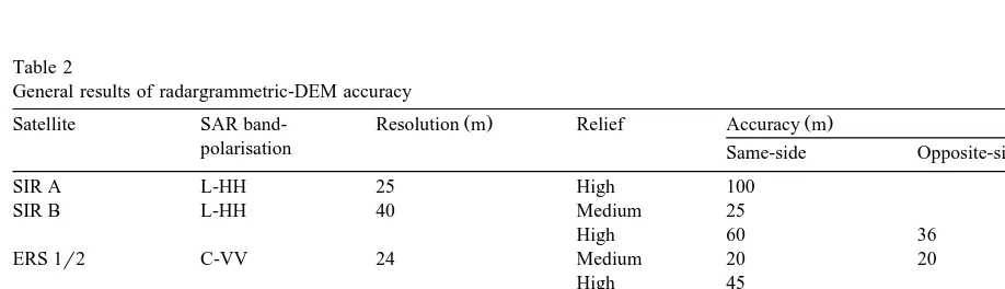
erties, geographic conditions, etc. . The advantages of one characteristic must be weighted against the deficits of the other. Table 2 summarises the general results of DEM generation with stereoscopy.
3.2. Combined sensors
Due to the increasing amount of sensors, it is very common to have data from different sensors over the same area. The traditional stereoscopic technique can be applied also with such data. By combining the different radiometry in the brain, the stereoscopic fusion of combined data can provide a virtual 3D
Table 2
General results of radargrammetric-DEM accuracy
Ž . Ž .
Satellite SAR band- Resolution m Relief Accuracy m
polarisation Same-side Opposite-side
SIR A L-HH 25 High 100
SIR B L-HH 40 Medium 25
High 60 36
ERS 1r2 C-VV 24 Medium 20 20
High 45
JERS L-VV 18 High 75
Almaz S-HH 15 High 30–50
a
RADARSAT C-HH F 7–9 Low 8–10 20
a
S 20–29 Medium 15–20 40
a
W 20–40 High 25–30
a
model of the terrain surface. Few results have been published on the use of combined stereo VIR and SAR sensors to generate DEMs.
Ž .
Moore 1969 first addressed the principle theoret-ically, by using simultaneously infrared line-scanner and SLAR images. The visual stereo effect was not perfect except near 458viewing angle. Various scal-ing factors were also applied to different areas of the stereopair to obtain a proper stereo effect for height determination. No quantitative measurement was re-alised due to the lack of an ‘‘adapted’’ stereo-plotter. Further evaluation has been realised with SIR-B
Ž .
and Landsat-TM images Bloom et al., 1988 . Ap-proximate error evaluation showed moderate results
Žin the order of 100 m for 27 extracted points sharp. Ž .
ridge crests , mainly due to image resolution, differ-ent object appearance, errors in the image registra-tion and the imprecise look angles used in the simplified elevation computation equation. Using a
Ž .
better parametric solution, Raggam et al. 1994 extracted a DEM from a multi-band SPOT and air-borne SAR stereopair. Since no meaningful results can be obtained from automatic image matching, they interactively measured 500 corresponding image points without stereoscopic capability and computed the elevation off-line. Results of the com-parison with a reference DEM showed a standard deviation of 60 m with a 42-m bias and minimumr maximum error of about "250 m. More recently,
Ž .
Toutin 2000b further investigated the mapping fea-sibility of combined sensor stereo-pairs with para-metric geopara-metric solutions ported to a digital stereo-workstation adapted to process on-line VIR and SAR
Ž
stereo-pairs. From the raw images no epipolar
re-.
sampling , the data are interactively extracted, and then directly compared to a checked DEM. An accu-racy of 20 m with no bias and minimumrmaximum errors of less than"100 m has been achieved from two different SPOT-PAN and ERS-SAR stereo-pairs: one being an opposite-side stereo-pair and the other a same-side stereo-pair. The full on-line stereo capa-bilities in the GCP plotting and elevation measure-ments account for the good results. Comparisons of the two stereo-pair results showed that the elevation parallax, which contributes to the determination of the elevation, is dominated mainly by the SAR ge-ometry with its high sensitivity to the terrain relief. Conversely, the SPOT-PAN images mainly
con-tribute to the easier identification of features, due to the better image quality and higher spatial resolution.
3.3. Processing, methods and errors
The different processing steps to produce DEMs using stereo-images can be described in broad terms:
Ž .i acquiring stereo-images; ii collecting GCPs andŽ . Ž .
stereo-model set-up; iii extracting elevation paral-laxes and computing 3D coordinates.
3.3.1. Acquiring stereo-image data
The SAR images are standard products in slant-or ground-range fslant-orms. They are generated digitally during post-processing from the raw signal SAR data
ŽDoppler frequency, time delay . The ground-range.
form is more popular, since the pixel spacing on the ground is roughly the same for the different look-an-gle images. This facilitates stereo-viewing and matching. The geometric modeling solution to com-pute the stereo-model and 3D intersection starts gen-erally either from the projection equations
gener-Ž
alised for different scanning sensors Leberl, 1972;
.
Toutin, 1995 , from the Doppler and range equations
ŽDowman et al., 1997; Sylvander et al., 1997 , or.
from the equations of radargrammetry based on the
Ž
radar image geometry Leberl, 1990; Raggam et al.,
.
1993 . More details on the physical principles, math-ematical formulations and differences of these three methods can be found in the given references.
3.3.2. Collecting GCPs and stereo-model set-up
Independently of the SAR geometric modeling used, some GCPs are needed to refine the stereo-model parameters with a least square bundle adjust-ment process in order to obtain a cartographic-stan-dard accuracy. With a geometric modeling solution
Ž .
such as defined in Section 3.3.1, few GCPs 1 to 4 are required. In an operational environment, their number will vary as a function of their accuracy. They should preferably be located at the border of the stereo-pair to avoid extrapolation in planimetry, and should cover the full terrain elevation range. Height control points and tie points can be added to strengthen the stereo geometry.
aerial image surveys, map digitising, etc. The image coordinates are measured interactively at the plotter or the computer monitor. Since some workstations do not have full stereoscopic capabilities, the image coordinates are then measured monoscopically. Im-age coordinate measurement errors can be large with
Ž .
a SAR stereopair ca. 1–2 pixels and influence the DEM accuracy. Due to the same-side geometry with
Ž .
small intersection angles 88 to 208 of SAR stereo-pairs, the propagation of the monoscopic measure-ment errors increases with shallower look-angles and
Ž .
smaller intersection angles Toutin, 1998 . Conse-quently, the DEM accuracy can decrease by 20% to
Ž
40%, depending on the stereo-pair geometry Toutin,
.
1999, 2000a . Stereoscopic measurement leads to more accurate image co-ordinates and elevations.
3.3.3. Extracting eleÕation parallax
Two methods can be principally used to extract the elevation parallax using image matching:
com-Ž .
puter-assisted visual or automatic methods. These two methods can be integrated to take into account the strength of each one.
The computer-assisted visual matching is an ex-tension of the traditional photogrammetric method to extract elevation data at a stereo-plotter. It requires full stereoscopic capabilities with 3D viewing de-vices to generate on-line the 3D reconstruction of the stereo-model, to capture and to edit in real-time 3D elevation features. More details on SAR stereo-work-stations and their 3D capabilities can be found in
Ž .
Dowman et al. 1992 .
To view the images in stereo, the images are resampled into an epipolar or quasi-epipolar geome-try, in which only the X-parallax related to the elevation is retained. Another solution to achieve stereo-viewing using the raw images is to automati-cally and dynamiautomati-cally remove the Y-parallax at the
Ž .
floating mark position Toutin, 1995 . Image mea-surement and computation of ground co-ordinates are performed as with conventional stereo-plotters.
Ž
Some automated tasks displacement of the images or cursors, prediction of the corresponding image
.
point position, etc. may be added.
However, computer-assisted visual matching to derive DEMs is a long and expensive process. Thus, when using digital images, automated image match-ing can be used. Since image matchmatch-ing has been an
active research topic for the last 20 years, an enor-mous body of research work and literature exists on stereo-matching.
The first generation of image matching methods is
Ž .
grey-level image matching Marr and Poggio, 1977 . Although satellite images are not like a random-dot
Ž .
stereogram easily matchable , grey level matching has been widely studied and applied to SAR data. Grey level matching can be computed with the
nor-Ž
malised cross-correlation coefficient Simard et al.,
.
1986; Sylvander et al., 1997 , the sum of mean
Ž
normalised absolute difference Ramapriyan et al.,
. Ž
1986 , a least squares solution Dowman et al.,
.
1997 , etc. The first one is considered to be the most
Ž .
accurate Leberl et al., 1994 and is commonly used with SAR images. Furthermore, a hierarchical strat-egy is sometimes implemented to reduce the SAR image noise and the elevation parallaxes, which en-ables to derive an approximate DEM at each image
Ž .
pyramid level Dowman et al., 1997; Toutin, 1999 . Marr also developed a second generation of image
Ž
matching: feature-based matching Marr and
Hil-.
dreth, 1980 . The same object may look considerably different in SAR images acquired at different times and with different geometric relationships between the SAR transmit and receive antenna and the ter-rain. But, according to Marr’s theory, image edges reflect generally true object structures. However, feature-based matching has not been very popular with SAR images because edges in mountainous terrain may differ a lot from one image to the other. Thus, hybrid approaches can be realised to achieve better and faster results by combining grey-level matching and feature-based matching with a hierar-chical multi-scale algorithm, but also with computer-assisted visual matching. The feature-based approach may produce good results for well-defined features, but no elevation values in-between. These results can then be used as seed points for grey-level matching. Another hybrid approach is to generate in a first step grey-value gradient images instead of binary edge images. Then, any grey-level matching technique can be used on these preprocessed images
ŽPaillou and Gelautz, 1999 . The linear gradient.
operator used by them was designed to be optimal to
Ž .
DEM reconstruction, not always significant or con-sistent, but at least with less blunders due to the noise removal.
Although the computer-assisted visual matching is a long process, it has been proven to be more
Ž
accurate with SAR data Leberl et al., 1994; Toutin,
. Ž
1999 or with combined sensors Raggam et al.,
.
1994; Toutin, 2000b . Thus, it could be used to add new points in areas with sparse measurements, elimi-nate blunders, and correct mismatched areas or areas
Ž
with errors larger than one pixel about 40% to 50%,
.
Leberl et al., 1994 . It could also be used to generate seed points for the automatic matching.
4. Interferometry
Radar interferometry is an alternative to the con-ventional stereoscopic method for extracting relative or absolute elevation information. It uses the coher-ent property of modern SAR and enjoys the advan-tages of radar systems and of digital image process-ing: all-weather, night and day operation, and auto-mated or semi-autoauto-mated processing. Imaging
inter-Ž .
ferometric SAR InSAR combines complex images recorded either by two antennas at different loca-tions, or with the same antenna at two different times
Žsee Fig. 2 bottom left . If the same antenna is used.
at two different times, then the location difference must be small, normally less than a kilometre for satellite repeat-pass interferometry. The phase differ-ence information between the SAR images is used to measure precisely changes in the range, on the sub-wavelength scale, for corresponding points in an image pair. Analysis of the differential phase, and therefore change in distance, between the corre-sponding pixel centres and the observing antenna can lead to information on terrain elevation or, with observations with the same antenna at different times, on terrain displacement.
Apart from airborne demonstration at the Jet
Ž .
Propulsion Laboratory JPL in Pasadena, USA, spaceborne SEASAT data was used by Li and
Gold-Ž .
stein 1990 to show the feasibility of combining data from pairs of passes for the derivation of height information. The technique was extended to SIR-B data acquired from two separate Shuttle passes
ac-Ž
quired over several days Gabriel and Goldstein,
.
1988 . The exciting early observation of in-scene relative movement was also made at JPL by Gabriel
Ž .
et al. 1989 , although the first quantitative demon-stration that millimetre scale movement is measur-able with radar interferometry was shown by Gray
Ž .
and Farris-Manning 1993 at the Canada Centre for
Ž .
Remote Sensing CCRS using airborne repeat-pass interferometry. After the launch of ERS-1 in 1991, numerous multi-pass satellite interferometric studies
Ž .
have been realised Massonnet and Rabaute, 1993 ,
Ž
subsequently with Almaz-1 Yelizavetin and
Kseno-. Ž
fontov, 1996 and with RADARSAT Geudtner et
.
al., 1997 . Although the early emphasis in the re-search with satellite InSAR data was on the estima-tion of terrain topography, there has been increasing work on use of InSAR techniques for measuring
Ž
terrain movement and change: with ERS-1r2 and
.
tandem mode data , SIR-C, RADARSAT, and with data from the Japanese satellite JERS-1. This work has been recently reviewed by Massonnet and Feigl
Ž1998 ..
With existing satellite SAR sensors, only the
re-Ž
peat-pass system one satellite antenna and two passes
.
of the satellite can generate interferometric data through the combination of complex images since there is presently no satellite system with two anten-nas. Such a dual-antenna system, the Shuttle Radar
Ž .
Topographic Mission SRTM , has been launched in early 2000. Although this system provides 100-m grid spacing DEMs of a large fraction of the Earth’s surface, in the following we concentrate on the methodology and accuracy of DEM generation using repeat-pass InSAR with existing satellite sensors.
Before outlining the processing stages in satellite repeat-pass InSAR, it is important to understand the conditions necessary for interferometry, and to be able to select pairs of passes that may have the necessary properties for the creation of useful geo-physical information. The imaging geometry of the first pass must be repeated almost exactly in the second pass. The concept of the critical baseline was
Ž
introduced Gabriel and Goldstein, 1988; Massonnet
.
ex-ceeded, one would not expect clear phase fringes or adequate ‘‘phase coherence’’. The sensitivity to ter-rain topography increases with the perpendicular baseline so that there is an optimum baseline for DEM generation. This is in contrast to the use of InSAR for terrain movement in which a very small baseline is clearly optimal to avoid problems with topography. In practice, the optimum baseline is terrain dependent as moderate to large slopes can generate an alias phase rate or a phase that can be difficult to process in subsequent stages such as phase unwrapping. Normally, a baseline between one
Ž
third and one half of the critical baseline i.e., around
.
300 to 500 m for ERS data is good for DEM generation, if terrain slope is moderate. In mountain-ous regions, a smaller baseline would be more appro-priate. RADARSAT has three options for the slant-range resolution, which are changed for the various
Ž .
modes Parashar et al., 1993 . In particular, use of the fine-resolution mode relaxes the criterion for the critical baseline and it is possible to use baselines of 1 km or even larger. This increases the sensitivity to topography and can lead to a more accurate DEM product than with the lower resolution modes of
Ž .
RADARSAT or ERS Vachon et al., 1995 .
Also, the difference in orientation of the imaging
Ž
planes the planes containing the line-of-sight and
.
vertical directions must be less than the azimuth beam width. This is most easily confirmed by check-ing the ‘‘Doppler parameters’’ used in the SAR data processing; there must be an overlap in the azimuth spectra. Orbit maintenance and attitude control of most satellites is such that this requirement is rarely a problem. It is possible to reduce the noise in the differential phase image through band-pass filtering
Ž
in both range and azimuth directions Prati and
.
Rocca, 1993 .
The complex SAR images are registered and the phase difference is computed for each pixel. Regis-tration can be accomplished in a number of ways, either based on cross-correlation of the image
ra-Ž .
diometry speckle correlation , or by optimising phase patterns or coherence for areas extracted from the two images. The product of one complex image times the complex conjugate of the second image is the primary product in InSAR work and is often referred to as an interferogram, although some au-thors prefer to use this term for a normalised product
or even a phase difference image. If the backscatter has not changed significantly over the time between acquisitions, the phase of the interferogram is not random but contains information on the differential range from the object pixel to the SAR antenna in the two passes. There is a stereoscopic component in the differential range that should be removed from knowledge of the orbit data. This is sometimes re-ferred to as the ‘‘flat Earth correction’’ stage. Fur-thermore, it is also advantageous to use even a coarse-resolution DEM to remove some of the phase variations due to topography. After the flat Earth and first order topographic corrections have been made to the phase of the interferogram, one can now carry out an averaging in the complex domain and be more confident that the process will not corrupt the phase. The averaged interferogram can be used to provide a multi-look image, as well as an image of a secondary product, i.e., the coherence. The maximum value for the coherence is 1, corresponding to all pixels in the window having the same phase. Unfortunately, the coherence depends on the size of the window used in
Ž .
its calculation Touzi et al., 1999 and the reader is cautioned in comparing quantitative values from dif-ferent experiments, unless the procedure is well de-scribed.
The phase of the averaged interferogram is known only between yp and qp. It is necessary to ‘‘unwrap’’ the phase difference to estimate how the differential range changes across the image. Often there are areas of lower coherence and higher phase noise, which lead to problems with phase unwrap-ping. One approach in avoiding the problem of error propagation when the phase is unwrapped incorrectly is to identify phase ‘‘residues’’. If one integrates the phase over a closed path, the sum of the phase values should be zero. If the value is closer to a multiple of 2p, this indicates a phase residue, and unwrapping across a line connecting adjacent residues should be
Ž .
avoided Goldstein et al., 1988 . Phase unwrapping remains an area of active research and many
ap-Ž
proaches have been suggested Ghiglia and Pritt,
.
phase noise can be blocked out and phase unwrap-ping completed around them.
The terrain elevations can be derived from the unwrapped phase, the baseline information,
beam-Ž .
pointing information from Doppler parameters , and
Ž .
an Earth model usually an ellipsoid . If an initial DEM is used to reduce the fringe rate and improve the range filtering for slopes, then of course the solution would be the additional topographic varia-tion. This process is often based on the SAR
geocod-Ž .
ing work of Curlander 1982 . In principle, the pro-cess can be completed without recourse to ground control points but in practice some ground control is important to reduce the need for precise orbit infor-mation. Control points are normally used to refine the baseline model used in the phase to height algorithm. The baseline is not constant for a scene, and usually the refinement can be modeled as a linear change in the vertical and horizontal direction. In one careful and systematic study of InSAR
de-Ž .
rived topography Small et al., 1995 , the accuracies for height determination were 2.7 m RMS for rela-tively small areas, a 12 by 13 km area close to Bonn, Germany, and only small biases were observed over a 40 by 50 km scene. However, the presence of different propagation conditions during data acquisi-tion can affect the differential phase and degrade the results. Small changes of the actual baseline can be used to compensate for different large-scale propaga-tion condipropaga-tions during the two acquisipropaga-tion dates
ŽTarayre and Massonnet, 1996 ..
Various propagation effects can corrupt the differ-ential phase and create errors in an interferometric product. These have been largely described by
vari-Ž
ous authors Goldstein, 1995; Massonnet and Feigl,
.
1995; Tarayre and Massonnet, 1996 . The usual culprit is variations in atmospheric water vapour in the troposphere, which retards the propagation and leads to an additional phase variation that corrupts interpretation of the differential phase in terms of topography or surface motion. Ionospheric effects
Ž
can also lead to InSAR errors Tarayre and
Masson-.
net, 1996 and are particularly important in the
auro-Ž .
ral zone of polar regions Gray et al., 2000 . Even tests of interferometric mapping in the high Arctic in winter have revealed modulations in a height error
Ž
map a comparison of airborne and spaceborne
In-.
SAR derived DEMs , which appeared to be related
Ž
to variations in atmospheric water vapour Mattar et
.
al., 1999 .
There are a number of approaches to both recog-nising these effects and in adopting a strategy to
Ž .
minimise the errors. Ferretti et al. 1999a show that combining multiple interferograms can improve the quality of a DEM product as well as simplify phase unwrapping. By looking for time coincident weather data it may also be possible to exclude passes which include heavy cumulonimbus clouds or rain. Another simple strategy is to work with as large a baseline as possible. In this way the phase error associated with the propagation inhomogeneity leads to a smaller error in elevation. This strategy was used to show the strength of RADARSAT fine mode InSAR in a dry Arctic environment in comparison to some ERS tandem modes pairs with much smaller baselines
ŽMattar et al., 1999 ..
Although propagation effects can limit the accu-racy with which a DEM can be generated with satellite SAR interferometry, the limitation imposed by temporal coherence is more fundamental. Coher-ence will vary with frequency and with time but experience with C-band data shows that the rate of coherence loss varies widely dependent on the
ter-Ž .
rain Zebker and Villasenor, 1992 . Even the C-band ERS tandem mode data with 1-day separation has not yielded good results for tropical rain forest, but other dry areas have shown coherence over very long
Ž
periods, on the order of 1 year Massonnet and Feigl,
.
1998 . As RADARSAT has a repeat cycle of 24 days, this represents a limitation for the exploitation of interferometry, although useful results have been
Ž .
obtained for dry terrain. Ferretti et al. 1999b have shown that using phase results from specific
‘‘per-Ž
manent scatterers’’ man-made structures, large
.
rocks, etc. that are stable can extend the time period over which useful measurements can be made, even if most of the scene has lost coherence usually due to vegetation and moisture change.
Current developments also include the use of satellite radar interferometry to study dynamic phe-nomena and their relative elevation displacement
Ždifferential interferometry . Combining a SAR inter-.
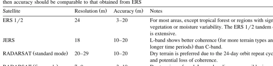
Table 3
Ž .
General results of interferometric-DEM accuracy. As with stereo SAR, results from low relief terrain lowest values will be better than
Ž .
those from areas with significant relief highest values , although no quantitative evaluation has been done on this topic. Quantitative tests of the accuracy of RADARSAT standard mode InSAR are somewhat limited, but when good coherence and suitable baselines are achieved, then accuracy should be comparable to that obtained from ERS
Ž . Ž .
Satellite Resolution m Accuracy m Notes
ERS 1r2 24 3–20 For most areas, except tropical forest or regions with significant vegetation or moisture variability. The ERS 1r2 tandem data archive is extensive.
Ž
JERS 18 10–20 L-band shows better coherence for more terrain types and for
.
longer time periods than C-band.
Ž .
RADARSAT standard mode 20–29 10–20 Dry terrain is preferred due to the 24-day orbit repeat cycle and potential loss of coherence.
Ž .
RADARSAT fine mode 7–9 3–10 Dry terrain preferred. Larger baselines are possible, increasing accuracy and reducing sensitivity to propagation effects.
Ž .
earthquake can be drawn Massonnet et al., 1993 . Topographic and displacement components can be also separated by combining three radar images to
Ž .
generate two interferograms Zebker et al., 1994 . The estimation of the displacement field using radar data alone, without any terrain information is then possible. Similarly, using repeat-track interferometry with a very small cross-track baseline, which gener-ates interferograms with little sensitivity to
topogra-Ž .
phy small topographic component , Goldstein et al.
Ž1993. measured and estimated ice sheet motion. This technique is currently applied with RADARSAT data from the Antarctica mapping mission to
mea-Ž .
sure ice motions Gray et al., 1998 and to analyse
Ž .
glacier flow dynamics Forster et al., 1998 .
So far, the atmospheric component and the image coherence are the main limitations of the interfero-metric method for operational DEM generation. The coherence image has also been used as SAR interfer-ometric signature for land-use classification with
Ž
ERS-1 SAR repeat-pass data Wegmuller
¨
and.
Werner, 1995 . The interferometric coherence over forested areas was found to be significantly lower than over open canopies, small vegetation, bare soils and urban areas. The results strongly support defor-estation studies, forest mapping and monitoring since it was possible not only to distinguish coniferous, deciduous and mixed forest stands, but also regrowth and clear-cut areas.
Although these results indicated that the scene coherence over forested areas was low, the interfero-metric technique can still be used to estimate the
topography and tree heights in specific conditions, such as a boreal forest in wintertime where the
Ž
coherence varied from 0.2 to 0.5 Hagberg et al.,
.
1995 . The interferometric phase information used to estimate the tree height relative to an open field and compared with in-situ measurements demonstrated that the scattering centre at C-band is close to the top of the trees if the forest is dense. The good coher-ence obtained is also a result of the stiffness of the ‘‘frozen’’ branches on the top of the boreal forest during the wintertime. They also noticed increased sensitivity of the degree of coherence to other
envi-Ž
ronmental parameters temperature, precipitation,
.
snowfall and soil moisture change . Table 3 sum-marises the general results of DEM extraction with interferometry. The accuracy figures given are an indication of the expected error range due to all sources: noise, baseline, propagation effects, etc. As with stereo SAR, results from low relief terrain
Žlowest values will be better than those from areas.
Ž .
with significant relief highest values although no quantitatively evaluation has been done. Quantitative tests of the accuracy of RADARSAT standard mode InSAR are somewhat limited, but when good coher-ence and suitable baselines are obtained, then accu-racy should be comparable to that obtained from ERS.
5. Polarimetry
scenes and man-made targets. A recently developed application of SAR polarimetry involves both a
di-Ž
rect measure of terrain azimuthal slopes see Fig. 2
.
bottom right and a derived estimate of the terrain
Ž .
elevations Schuler et al., 1996 . The method is mainly based on empirical comparisons, supported by preliminary theoretical analysis, between the ter-rain local slope and the co-polarised signature maxi-mum shift. This has been validated over different geographical areas and different types of natural targets using different DEMs as reference. Although it was only tested with airborne P- and L-band SAR platforms, it is worth mentioning since future
satel-Ž .
lite missions RADARSAT-2 will generate full po-larimetric SAR data.
Polarimetric SAR measures the amplitude and phase terms of the complex scattering matrix. Based on a theoretical scattering model for tilted, slightly
Ž .
rough dielectric surfaces Valenzuela, 1968 , az-imuthal surface slope angles and signature-peak ori-entation displacements produced by such slopes are proportional over a range of azimuthal slopes. Schuler
Ž .
et al. 1993 first demonstrated that the resolved azimuthal wave-tilts produced significant and pre-dictable displacements in the location of the maxima of the co-polarised signature of ocean backscatter. They then hypothesised that an azimuthal angle of an open-field terrain caused a proportional shift of the co-polarised polarimetric signature maximum from its flat position by an angle almost equal to the terrain slope. Azimuthal direction slopes can then be computed from the polarimetric SAR data without any prior knowledge of the terrain. By integrating the slope profiles in the azimuthal direction, relative terrain elevation can be derived. To obtain absolute elevation, one elevation point must be known along each slope profile.
Since forest scattering is more complex than open-field terrain scattering, radiative transfer
mod-Ž
els or discrete scatter formulations Durden et al.,
.
1989 of forest backscatter from a sloping terrain have to be used to modify the open-terrain algorithm.
Ž .
Schuler et al. 1996, 1998 carried out experiments with airborne NASArJPL AIRSAR polarimetric
P-Ž
band SAR data resolution 6.6 m in range by 12.1 m
.
in azimuth, 4 looks over forested areas and medium
Ž
relief terrain slopes of generally 08 to 58 but up to
. Ž .
308. Digital surface models DSMs , which take into
account the canopy height, are used as reference data, and also to provide the starting elevation point for each azimuth profile. Accuracies of 38 to 58 and
Ž
20 to 30 m with high correlation coefficients 0.8–
.
0.9 were obtained for the slopes and elevations, respectively. They are correlated with the terrain
Ž .
relief: for the lowest 08 to 58 slopes and highest Ž158to 258slopes relief, accuracies of 8 to 20 m and.
30 to 40 m were obtained, respectively. The canopy height may not account for part of these errors, since the elevation of ‘‘starting’’ points for each profile to integrate the slopes into elevations have been
ex-Ž .
tracted from DSMs including the canopy height . Furthermore, attempts to use shorter wavelength
Ž .
radars C- or L-band yielded profiles with larger errors for forested terrain, mainly for the C-band
ŽSchuler et al., 1996 . The larger slope error indi-.
cates that canopy andror branch scattering is then dominant over the terrain relief scattering.
The technique has also been applied with AIR-SAR L-band AIR-SAR data over flat desert terrain with
Ž
some rugged mountains 500 m elevation range with
. Ž
up to 508 slopes devoid of trees Schuler et al., .
1996 . To be representative of an open-field terrain, a simplified closed form approximation to the rela-tionship between the co-polarised maximum shift and the measured co-variance matrix elements is first established. Co-variance matrices generated from ex-perimental or modelling data can then be used as input parameters to derive the link with the terrain azimuthal slope. Two azimuthal profiles were com-pared to a very accurate DEM, which is also used to integrate the elevation along profile. The achieved accuracies were 2.58to 3.58and 6 m to 24 m for the slopes and elevation, respectively; the lowest values for the desert terrain and the highest ones for the mountain range.
Since a DEM is not normally available in an operational environment when applying this method, sets of elevation profiles spaced throughout the range direction have to be available to obtain two-dimen-sional topographic elevations maps. Two orthogo-nal-pass SAR data is thus a solution to generate an elevation surface with only one elevation point
ŽSchuler et al., 1998 . The elevation surface may be.
Ž
desert terrain with some mountain range 400 m
.
elevation range having little ground cover, DEM results showed an accuracy of 29 m. However, a 6-m accuracy was achieved in the flat desert terrain. Part of these errors was caused by registration errors and by significant changes in data quality between the two passes. Since these last results are about the same as those obtained from one pass, the two-pass technique is mainly useful to reduce the number of elevation tie-points to one. Furthermore, orthogonal passes cannot be obtained with sun-synchronous
Ž .
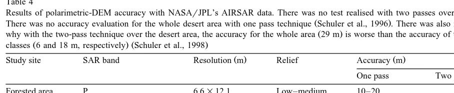
satellites except close to the poles . Shape-from-shading techniques, which generate slopes in the across-track direction, could then be another solu-tion. Table 4 summarises the general results of eleva-tion extraceleva-tion or DEM generaeleva-tion with polarimetry, only from airborne SAR data.
Ž
However, to apply this technique one pass or two
.
quasi-orthogonal passes with satellite SAR data
Žmainly C-and X-bands , future work should be di-.
rected towards an analysis based on a volume scat-tering to take into account the more complicated situation of the SAR backscattering in forested or agricultural areas. With such scattering models, quantitative slope and elevation values could be de-rived from the relationship between radiation fre-quency, incidence angle and type of scatterer. How-ever, the main drawbacks of this emergent technique are the volume scattering models but also the limited availability of polarimetric data to evaluate the ro-bustness of the technique with different topographic and land-cover situations.
6. Concluding remarks
Elevation modeling from satellite data has been an active R & D topic in the theoretical development for the last 30 years and in the practical experiments for the last 20 years with the appearance of the first civilian remote sensing satellite. SAR data in
differ-Ž .
ent formats analogue but mainly digital can be
Ž
processed by different methods clinometry,
stere-.
oscopy, interferometry, polarimetry taking advan-tage of the different sensor and image characteristics
Žgeometric, radiometric, phase using different types.
Ž .
of technology analogue, analytical, digital and
pro-Ž .
cessing interactive, automatic .
Most of the techniques have been proposed and addressed in the early years. However, the limited availability of data and associated technologies has restricted their evolution in comparison to traditional photogrammetry. Their respective evolution is a function of the research effort in terms of physical parameter modeling and data processing.
The shadowing method, providing localised cues along special contours is principally used to derive relative elevation of a specific target. Despite good results, the method remains limited to specific appli-cations. Conversely to shadowing, shading provides cues all over the studied surface, but can be applied successfully only with homogeneous surfaces. Com-bined with the empirical approach to resolve the different ambiguities, this method also remains marginal, whatever its potential accuracy. Both methods have generated limited interest in the
scien-Table 4
Results of polarimetric-DEM accuracy with NASArJPL’s AIRSAR data. There was no test realised with two passes over forested area.
Ž .
There was no accuracy evaluation for the whole desert area with one pass technique Schuler et al., 1996 . There was also no explanation
Ž .
why with the two-pass technique over the desert area, the accuracy for the whole area 29 m is worse than the accuracy of the other relief
Ž . Ž .
classes 6 and 18 m, respectively Schuler et al., 1998
Ž . Ž .
Study site SAR band Resolution m Relief Accuracy m
One pass Two passes
Forested area P 6.6=12.1 Low–medium 10–20
High 30–40
Whole area 20–30
Ž . Ž .
Desert area L 1 pass P 2 passes 6.6=12.1 Low–medium 6 6
High 24 18
tific community. On the other hand, stereoscopy is the most preferred and used method in the mapping, photogrammetry and remote sensing communities, most likely due to the heritage of the well-developed stereo-photogrammetry. Advances in computer vi-sion to model human vivi-sion has led to the advent of new automatic image processing approaches applied to satellite stereoscopy. It has thus allowed the map-ping process to become more automated, but not completely due to occasional matching failures. In-versely, radar polarimetry stays mainly at the level of scientific interest on the physical parametric model-ing without much effort on data or image processmodel-ing development.
Their evolution in relation to the scientists’ inter-est is also a function of the predominant ‘‘fashion’’. SAR stereoscopy was popular around the 1980s with the development of radargrammetry equations and the first interesting and promising results with SIR-B. However, the SAR image processing and related
Ž
technologies to extract elevation data such as image
.
matching were not mature enough and led to a temporary decline. In the same way, most of the R & D in shape-from-shading methods were per-formed in the 1980s starting with the Venus radar mapper. Similar developments applied to SPOT data took place at that time, with enormous research around the world both for physical parametric mod-eling and image processing, taking also advantage of the R & D in digital photogrammetry.
When ERS-1 was launched, scientists became enthusiastic over interferometric techniques because of the apparent high accuracy for DEM extraction. In the first years, most of the research efforts have focused on image processing, particularly phase un-wrapping, and few on the problems of atmospheric propagation and use of height control.
With the launch of RADARSAT in 1995, radar-grammetry experienced a revival of the scientists’ interest, taking advantage of the R & D on image matching realised for SPOT at the end of the 1980s and the new computer technologies. R & D at the dawn of the next millennium will be focused on the use of the high-resolution SAR satellites and the development of their associated technologies, such as ENVISAT, RADARSAT-2 and the SRTM.
Since any sensor, system or method has its own advantages and disadvantages, solutions to be
devel-oped in the future for operational DEM generation should use the complementarity between the differ-ent sensors, methods and processing. It has already been used in stereoscopy combining VIR and SAR data, where the radiometric content of the VIR image is combined with the SAR high sensitivity to the terrain relief and its ‘‘all-weather’’ capability to ob-tain the second image of the stereopair.
Based on the same philosophy, other complemen-tary sensor data can be used.
Ž .1 Two SAR stereoscopic pairs from ascending and descending orbits to partially complement shadow and layover areas of each stereopair.
Ž .2 Two interferometric pairs, one with a small
Ž .
baseline to help the phase unwrapping , and the
Ž
other with a larger baseline to increase the
accu-.
racy .
Ž .3 Two polarimetric images from ascending and
descending orbits to resolve the across-track ambigu-ity and reduce the required number of known eleva-tion points.
The complementarity of methods has already been tried with SAR where stereoscopy is used to gener-ate seed points needed for the clinometry or to generate an approximate DEM to help the phase unwrapping in interferometry. The loss of coherence with interferometry in forested areas can be comple-mented with clinometry, which is well suited to the homogeneity of the forest cover. Clinometry and polarimetry could be combined since the first one gives elevation information in the range direction and the second one in the azimuthal direction. Only one polarimetric SAR image could thus be neces-sary. A shadow-based method to extract building or tree heights could also be used to transform a stereo-scopic or interferometric DSM into a DEM, or the reverse.
The complementarity can also be applied at the
Ž .
processing level: i using visual matching to mea-sure seed points for the automatic matching or to
Ž
post-process and edit raw DEMs occlusion, shadow
. Ž .
or mismatched areas , or ii using stereo
measure-Ž
ments of geomorphologic features thalweg and crest
.