Environmental Computable General-Equilibrium
Approach for Developing Countries
Jian Xie and Sidney Saltzman, Department of City and Regional Planning, Cornell University
Environmental pollution is now a serious problem in many developing countries. One approach to combat the problem is to implement various pollution control policies. How-ever, due to a lack of adequate quantitative models, the economic impacts and effectiveness of many pollution control policies are still unknown.
This article uses the computable general-equilibrium (CGE) approach to develop an integrated economic and environmental model for environmental policy analysis for devel-oping countries. The model presented here incorporates various environmental compo-nents, including pollution taxes, subsidies, and cleaning activities, into a standard CGE framework. The study also presents an environmentally extended social accounting matrix (ESAM), which serves as a consistent data set for calibrating the model.
The model is applied to China, the largest developing country in the world, for evaluating the effectiveness of Chinese environmental policies on pollution control and their impacts on the Chinese economy. The environmental policies under scrutiny include pollution emission taxes and pollution abatement subsidies. The economic impacts of the waste water treatment plan in China’s recently launched five-year environmental protection
Address correspondence to Jian Xie, The World Bank, Rm. J4-010, 1818 H Street, N.W., Washington, DC 20433.
Prepared for presentations at the Sixth International CGE Modeling Conference, Octo-ber 1995, University of Waterloo, Ontario, Canada, and at the 42nd North American Meetings of the Regional Science Association International, November 1995, Cincinnati, Ohio, USA.
The authors would like to thank Professors Iwan Azis, Walter Isard, and Erik Thorbecke at Cornell University for their suggestions and comments. In addition, the first author is grateful to Keith Florig, Raymond Kopp, and Walter Spofford at Resources for the Future; Shantayanan Devarajan, Jeffrey Lewis, John O’Connor, and Zhi Wang at the World Bank; Richard Garbaccio at the East–West Center; Theodore Panayotou at the Harvard Institute for International Development; Christian Dufournaud at Waterloo University; and Dianq-ing Xu at the University of Western Ontario; for their interests and helps in the research and helpful discussions on this topic. The views expressed are solely those of the authors.
Received March 1996; final draft accepted November 1996.
Journal of Policy Modeling22(4):453–489 (2000)
program are also examined. 2000 Society for Policy Modeling. Published by Elsevier Science Inc.
1. INTRODUCTION
Environmental problems are serious and pervasive in today’s world. In many developing countries, industrial pollution emis-sions continue to increase and, as a result, environmental prob-lems, such as deforestation, soil erosion, and the expansion of desert areas, are aggravated. These problems have severely threat-ened the sustainable development of these countries and have caused great concern at all levels, from the general public to national governments and international agencies.
Because they face serious environmental degradation, the gov-ernments of many developing countries have begun to introduce environmental policies and regulations to combat environmental problems. The most popular environmental policies include pollu-tion taxes, environmental impact assessments, pollupollu-tion subsidies, and pollution emission permits. However, due to a lack of ade-quate quantitative models for environmental policy analysis, the effectiveness of pollution controls and the economic impacts of these policies are still unknown. Therefore, there is a strong need for analytical models for environmental policy analysis.
This article consists of six sections. Following this introductory section, Section 2 reviews the literature in environmental CGE models. Section 3 develops an environmental CGE model. It be-gins with an introduction to the interactions between production and pollution. The theoretical framework of a multi-sector envi-ronmental CGE model is then developed in this section. Section 4 introduces the framework of an environmentally extended social accounting matrix (ESAM). The ESAM serves as a consistent equilibrium data set for parameter calibration of the environmen-tal CGE model.
The application of the environmental CGE model to China using 1990 Chinese data is presented in Sections 5. Several Chinese environmental policy alternatives are simulated in this section, and the major findings from these policy simulations are discussed. Section 6 contains concluding remarks.
2. CGE MODELING FOR ENVIRONMENTAL POLICY ANALYSIS: THE LITERATURE
Due to its salient features mentioned in introduction section, CGE modeling emerged in 1960 (Johansen, 1960), and since the 1980s it has become a leading tool in the multi-sector, economy-wide modeling for policy analysis.
Studies on incorporating environmental components into a CGE framework emerged in the late 1980s. Forsund and Strom (1988), Dufournaud et al. (1988), Bergman (1988), Hazilla and Kopp (1990), Robinson (1990), and Jorgenson and Wilcoxen (1990) contributed to the early development of environmental CGE models. So far, about twenty stylized or applied environmen-tal CGE models have been described in the literature. These models, in one way or another, endogenize pollution effects into production or utility functions. These models have been applied mainly to environmental and economic impact assessments of various public policies, such as tax and government spending.
More recently, we have seen the rapid growth of CGE applica-tions in the arena of environmental policy analysis.1These CGE
models are distinct from each other in terms of the ways they integrate environmental components with economic activities in their CGE models. Environmental CGE models can be divided into several types according to the level of pollution-related activi-ties integrated into them. The first type of models is not very different from a standard CGE model.2They actually are extended
applications of standard CGE models. These extensions to stan-dard CGE models include either estimating pollution emissions using fixed pollution coefficients per unit of sectoral outputs or intermediate inputs,3or exogenously changing prices or taxes
con-cerning environmental regulations without any changes in model structure.4 To extend the applications of a standard CGE model
in such ways do not affect the behavioral specification of a standard CGE model, but only provide more detailed description of produc-tion results from the environmental prospective.
The second type of environmental CGE models, however, be-gins to introduce environmental feedback into economic systems. The models of this group, represented by Jorgenson and Wil-coxen’s (1990) model, have pollution control costs specified in production functions. A further extension of production specifica-tion is to consider the effects of environmental quality on produc-tivity.5To represent the effects of pollution emission and
abate-ment activities on consumption, a number of models have environmental effects incorporated in utility functions.6
Besides these modifications to production and consumption functions, a few models specify the production functions of pollu-tion abatement activities or pollupollu-tion abatement technologies. Robinson (1990) uses a Cobb–Douglas production function to represent a pollution cleaning activity. Nestor and Pasurka (1995) model air pollution abatement processes and abatement tax rates based on an augmented input–output table which represents the inputs purchased for air pollution abatement activities. Robinson
2The word “standard” is somewhat vague. However, it is used in the literature. A standard CGE model pretty much means the type of CGE models developed by the World Bank for developing countries to study structural change and international trades.
3The models of Blitzer et al. (1993), Lee and Roland-Holst (1993), and, Beghin et al. (1994) belong to this group.
4See, for example, Boyd and Uri (1991).
5See Bergman (1993), and Gruver and Zeager (1994).
et al. (1993) identify polluting production processes and abatement technologies of each process.7
Although there are diverse CGE models being applied to envi-ronmental policy analysis, envienvi-ronmental CGE modeling is still in its early stages. This is due to two reasons. The first is a relatively incomplete and unsophisticated specification of models of eco-nomic and environmental interactions. In many models, environ-mental externalities are weakly defined under rigid assumptions or exogenously determined, which undermines the effectiveness and comprehensiveness of an environmental CGE model. The second reason is a lack of a well-defined environmental data frame-work which can provide a solid basis for numerical specification of an environmental CGE model. In addition, most of the existing environmental CGE models are still stylized and ad hoc in nature. Even though a few models are applied to environmental issues in the real world, these models have mostly been built for developed countries. Few models aim at environmental issues of developing countries.
3. INTEGRATING ENVIRONMENTAL ACTIVITIES INTO A GENERAL EQUILIBRIUM FRAMEWORK: AN ENVIRONMENTAL CGE MODEL
This section summarizes the technical specification of an envi-ronmental CGE model developed by the authors. The model aims at simulating environmental policies and environmental protec-tion programs, such as polluprotec-tion taxes and environmental stan-dards, in developing countries.
3A. Economy-Environment Interactions: Diagrams
As mentioned earlier, the classical CGE approach assumes profit-maximizing producers and utility-maximizing consumers.
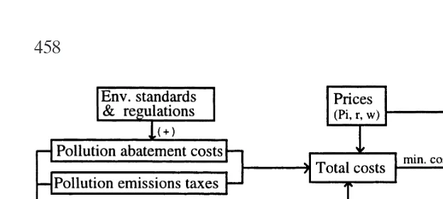
Figure 1. The pollution-production interactions.
Consumers’ and producers’ optimal behaviors are affected, in one way or another, by the effects of pollution emissions on production and consumption and the implementation of pollution control policies.
On the production side of the CGE model, each producer deter-mines his optimal output level by minimizing the costs of his inputs and maximizing the profits of his outputs. When pollution occurs in production processes and certain pollution emissions taxation, are required, the profit maximization problem of the producer is subject to changes. The producer will adjust his output level based on new costs and new production functions containing pollution effects. Figure 1 illustrates the impacts of pollution on production. First, Figure 1 shows that the producer’s total cost includes not only the costs of factor inputs but also pollution related costs due to environmental protection requirements. There are two types of pollution control costs specified in the figure. One is the pollution emission taxes and another the costs of removing pollution in order to comply with environmental standards. Here, no changes in production technology under pollution control requirements are assumed. Second, pollution, in many cases, affects productivity directly. Pollution emissions degrade environmental quality, which then affects the quality and quantity of production factors: fixed capital, labor, and land. The degradation of fixed capital and labor causes productivity to decrease.
How about the consumption side of the model? Without pollu-tion effects, household demands for two goods, C1and C2, in the
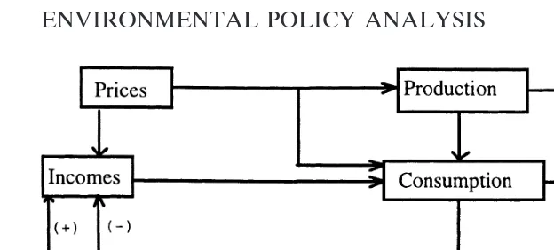
Figure 2. The pollution-consumption interactions.
However, when pollution occurs, it influences the household’s decisions on consumption. The interactions among pollution, pol-lution control and consumption are described in Figure 2.
Figure 2 shows two types of possible impacts of pollution on the consumption side of an economy: the decrease of utility and the changes in household disposable income. The household suf-fers from environmental degradation caused by consumption and production pollution emissions. Therefore, the more pollution the household “consumes,” the less utility it has. Two possible effects of pollution control activities on household disposable income are also identified in Figure 2. The first is the payment of the household for disposing of its waste. The payments for trash tax and motor vehicle waste gas emission tax are two common types of this kind. The second is a nominal increase of household through polluters’ compensating the environmental damage to the household. For example, a farmer may get compensation from a factory that discharges waste water into his farmland.
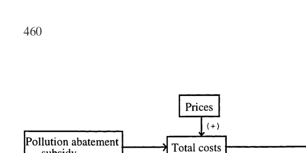
Figure 3. A pollution abatement sector.
To eliminate pollution as a result of satisfying pollution emission requirements, pollution abatement is required in many economies. Figure 3 depicts a representative pollution abatement sector.
Different from a production sector, the output of a pollution abatement sector (Ag) is the value of the pollution cleanup.
Pollu-tion cleanup can be viewed as special goods which are purchased at a certain price by polluters in order to reduce their pollution emission levels. The optimal output level of a pollution abatement sector can be determined in the way same as that of a production sector. The price of a pollution abatement service is assumed to be determined implicitly by the market. Such an assumption is likely true in a situation where pollution is treated in profit-seeking waste treatment plants, such as a private-owned waste water treat-ment plants. However, this assumption is unrealistic when pollu-tion abatement facilities or sectors are affiliated with an individual factory, because the in-built pollution abatement sectors or facili-ties will not likely pursue a maximum profit strategy on their own. When this is the case, we can fix the price of a pollution abatement service at the level of the average cost of the pollution abatement activity.
3B. General Features of the Model
countries.8Specifically, it is an adapted version of the Cameroon
models developed by Condon et al. (1986) and Devarajan et al. (1991).9However, the model presented here is unique in the way
it integrates various pollution control activities with economic activities in a CGE framework. The environmental part of this model includes mainly: (1) pollution abatement activities and pol-lution abatement costs (or payments) of production sectors; (2) pollution taxes, such as production pollution emission taxes and household waste disposal taxes; (3) pollution control subsidies; (4) environmental compensation; (5) separately accounted envi-ronmental investment; and, (6) various pollution indicators includ-ing pollution cleanup ratios and the levels of pollution abatement and emissions. The model can be characterized as an integrated economic and environmental model in the line of the CGE ap-proach.
The model assumes an economy having n production sectors and a representative household group. There are m types of pollutants generated from production and consumption processes and m pollution abatement sectors, each of which treats only one unique type of pollution. Production and pollution abatement sectors need intermediate inputs and two primary factors: capital and labor. Government and trades with the rest of the world are included in the model. The model is static with aggregate factor supplies exogenously determined.
Following closely the notation convention used in Devarajan, Lewis and Robinson’s model, the model presented here adopts (1) upper case letters for endogenous variables, (2) Greek letters or lower case letters for parameters, and (3) upper case with bar or lower case for exogenous or control variables. The indices for sets used in the model are:ip and jp 5 1, 2, . . . n, representing production sectors;gand ia51,2, . . .m, representing pollutants and pollution abatement sectors; and,iandj51,2, . . . ,n,n11, . . . ,n1m, containing both production and pollution abatement sectors. They appear as lower case subscripts.
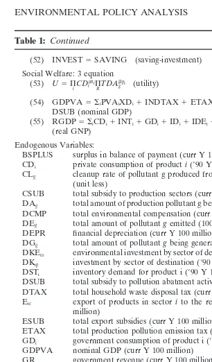
The model has over 50 equations or equation groups. They are divided into eight equation blocks. They are presented in Table
8These kinds of CGE models for developing countries were pioneered by, among others, Adelman and Robinson (1978), Taylor (1979), and Dervis et al. (1982).
1. A list of variables and parameters with units (used in the case study for China) is also enclosed in the table. A brief description of the model by equation blocks is provided below.10
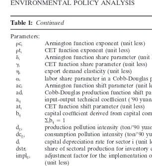
3B-1. Price Block. There are a total of ten different groups of average prices in the model. They are composite good prices (P), domestic good prices (PD), capital input prices (PK), the domestic process of imports and exports (PM and PE), the prices of intermediate inputs (PN), value-added prices (PVA), the world prices of imports and exports (PWM and PWE), and output prices (PX). The relationships among these prices are sketched in Figure 4, and the equations defining prices in the model are presented in block 1 of Table 1.
All of these equations in the price block, except for Equation 5, are standard in the literature of CGE models. Equation 5 shows the composition of production cost. The left-hand side of the equation is the total cash inflow of a sector, i.e., the product sale income plus the receipt of government subsidy. It is decomposed on the right-hand side into value-added prices (PVA), indirect taxes (tc), spending on intermediate inputs (based on the fixed input–output (I/O) coefficients ajp,i), pollution emissions taxes
(PETAXg,i) and pollution abatement costs (PACOSTia,i).
PE-TAXg,iand PACOSTia,iare affected by pollution intensities, pollu-tion cleanup rates and prices. They are defined later in Equapollu-tions 36 and 37 in pollution equation block.
The trade-related prices in the non-tradable sectors are set to zero, so are the prices for trade-related variables in the pollution abatement sectors because no pollution abatement services are assumed to be tradable. Finally, notice that the prices of pollution abatement services (PXiand PiiPia) are defined in this block in the same way as product prices.
3B-2. Output and Factor Inputs. For simplicity, production is modeled by a Cobb–Douglas production function of two primary factors (capital and labor) in Equation 8.11 The model assumes
that a firm maximizes its profits by hiring capital and labor until
10Again, space limitations preclude a more detailed discussion of the full model, see Xie (1995) in detail.
Table 1: An Environmental Computable General-Equilibrium Model
The model contains
nproduction sectors, of whichssectors export products andtsectors import goods; mtypes of pollution andmcorresponding pollution-abatement sectors;
two primary factors: capital (K) and labor (L), and intermediate inputs; one household group (h);
government (G); and, the rest of the world (ROW).
The following environmental components are incorporated into the model costs (or payments) of production sectors for pollution cleaning services, pollution abatement activities,
pollution emission taxes of production sectors, household waste disposal taxes,
environmental compensation by production sectors to household, and separately accounted environmental investment.
Sets
ip, jp51,2, . . .n. (production sectors)
g, ia51,2, . . .m. (pollutants or pollution abatement sectors)
i, j51,2, . . .n,n11 . . . n1m. (production and pollution abatement sectors) ie51,2, . . .t. (sectors with exports)
im51,2, . . .s. (sectors with imports)
ic51,2, . . .k. (sectors providing goods for final consumption) Equations SgPACOSTg,i (activity cost composition)
(6) PKi5 SjPjbj,i (price for capital input) (7) PINDEX5GDPVA/RGDP (price index)
Output and factor and trade: 3(n1m) equations
(8) XDi5adiKl-iaLai (Cobb-Douglas production function) (99) wldistiWL5 aPVAiXDi/Li (wage and labor demand)
(9″) wkdistiWK5(1-a)PVAiXDi/Ki (capital return and capital demand) Trade: 2(n1m)1t1s equations
(10) Xi5aci{diM2ipci1(12 di)XXD2ipci}21/pci (Armington function) (11) Mi5XXDi{(PDi/PMi)di/(12 di)}1/(11pci) iPim (import demand)
(12) XDi5ati{giEptii 1(12ci)XXDptii}1/pti (CET function)
(13) Ei5XXDi{(PEi/PDi)(12 gi)/gi}21/(12pti) iPie (export supply)
Income, Tax and Saving: 15 equations (14) Y5YH1YC (total income)
(15) YH5 SiwldistiWLLi (household labor income)
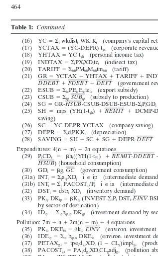
Table 1: Continued
(16) YC5 SiwkdistiWK Ki (company’s capital return) (17) YCTAX5(YC-DEPR) tyc (corporate revenue tax) (18) YHTAX5YC tyh (personal income tax)
(19) INDTAX5 SiPXiXDitci (indirect tax) (20) TARIFF5 SimPMimMimtmim (tariff)
(21) GR5YCTAX1YHTAX1TARIFF1INDTAX1ETAX1DTAX1
DDEBT1FDEBT1DEFT (government revenue) (22) ESUB5 SiePEieEieteie (export subsidy)
(23) CSUB5 SipSUBip (subsidy to production)
(24) SG5GR-HSUB-CSUB-DSUB-ESUB-SiPiGDi (government saving) (25) SH 5 mps (YH(1-tyh) 1REMIT 1 DCMP-DTAX-DDEBT) (household
saving)
(26) SC5YC-DEPR-YCTAX (company saving) (27) DEPR5 SidiPKiKi (depreciation)
(28) SAVING5SH1SC1SG1DEPR-DEFT (total saving) Expenditures: 4(n1m)12n equations
(29) PiCDi 5 bhi((YH(1-tyh) 1REMIT-DDEBT1DCMP-DTAX)(1-mps) 1
HSUB) (household consumption)
(30) GDi5 bgiGC (government consumption)
(31a) INTi5 Sjai,jXDj iPip (intermediate demand for goods)
(31b) INTi5 SjPACOSTi,j/Pi iPia (intermediate demand for pollution cleanup)
(32) DSTi5dstriXDi (inventory demand)
(33) PKipDKip5 bKip(INVEST-SiPiDSTi-EINV-BSPLUS) (nominal investment by sector of destination)
(34) IDip5 Sjpbip,jpDKjp (investment demand by sector of origin)
Pollution: 7m1n12m(n1m)14 equations
(35) PKiaDKEia5 bkiaEINV (environ. investment by sector of destination) (36) IDEip5 Siabip,iaDKEia (environ. investment demand by sector of origin) (37) PETAXg,i5tpegdg,iXDi(12CLg)implg,i (production pollution emission tax) (38) PACOSTg,i5PAgdg,iXDiCLgadjg,i (pollution abatement cost)
(39) PAg5(X0g/TDA0g)Pg (pollutant abatement price conversion) (40) TDAg5XgTDA0g/X0g (total pollution abated)
(41) DAg5TDAg-GDgTDA0g/X0g (production pollution abated) (42) CLg5DAg/Sidg,iXDi (cleanup rate for production pollution) (43) DGg5 Sidg,iXDi1 Sidcg,i(CDi1GDi) (total pollution generated) (44) DEg5DGg-TDAg (total pollution emitted)
(45) ETAX5 SiSgPETAXg,i (production pollution emission tax) (46) DTAX5 SgtpdgSipdcg,ipCDip (consumption waste disposal tax) (47) DSUB5 SiaSUBia (subsidy to pollution abatement)
(48) DCMP5 SgwgDEg (environmental compensation)
Market Clearing: (n1m)14 equations
(49) Xi5CDi1INTi1GDi1IDi1IDEi1DSTi (commodity equilibrium) (509) SiLi5LS(1-Runemp) (labor market equilibrium)
(50″) SiKi5KS (capital market equilibrium)
(51) SimPMimMim1BSPLUS5 SiePEieEie1REMIT1FDEBT (balance of payment)
Table 1: Continued
(52) INVEST5SAVING (saving-investment)
Social Welfare: 3 equation
(54) GDPVA5 SiPVAiXDi1INDTAX1ETAX 1 TARIFF-ESUB-CSUB-DSUB (nominal GDP)
(55) RGDP5 SiCDi1INTi1GDi1IDi1IDEi1DSTi)1 SieEie-SimMim(1-tmim) (real GNP)
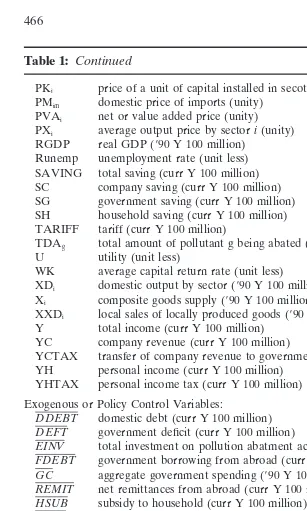
Endogenous Variables:
BSPLUS surplus in balance of payment (curr Y 100 million)* CDi private consumption of producti(990 Y 100 million) CLg cleanup rate of pollutant g produced from production sector i
(unit less)
CSUB total subsidy to production sectors (curr Y 100 million)
DAg total amount of production pollutant g being abated (100 million tons) DCMP total environmental compensation (curr Y 100 million)
DEg total amount of pollutantgemitted (100 million tons) DEPR financial depreciation (curr Y 100 million)
DGg total amount of pollutantgbeing generated (100 million tons) DKEia environmental investment by sector of destination (990 Y 100 million) DKip investment by sector of destination (990 Y 100 million)
DSTi inventory demand for product i (990 Y 100 million)
DSUB total subsidy to pollution abatment activities (curr Y 100 million) DTAX total household waste disposal tax (curr Y 100 million)
Eie export of products in sector ito the rest of the world (990 Y 100 million)
ESUB total export subsidies (curr Y 100 million)
ETAX total production pollution emission tax (curr Y 100 million) GDi government consumption of product i (990 Y 100 million) GDPVA nominal GDP (curr Y 100 million)
GR government revenue (curr Y 100 million)
IDEip environmental investment demand by sector of origin (990 Y 100 million)
IDip production investment demand by sector of origin (990 Y 100 million) INDTAX indirerct tax (curr Y 100 million)
INTi intermediate demand by sector of origin (990 Y 100 million) INVEST total investment (curr Y 100 million)
Ki capital demand by production sector i (990 Y 100 million) Li labor demand by production sectori(million workers)
Mim import from the rest of the world to the sector i (990 Y 100 million) PACOSTg,i pollution abatement costs (curr Y 100 million)
PAg price of pollutantgabated (curr yuan/ton) PDi domestic prices (unity)
PEie domestic price of exports (unity)
PETAXg,i pollution emission taxes (curr Y 100 million) Pi price of composite goodi(unity)
PINDEX GDP deflator (unity)
Table 1: Continued
PKi price of a unit of capital installed in secotri(unity) PMim domestic price of imports (unity)
PVAi net or value added price (unity) PXi average output price by sectori(unity) RGDP real GDP (990 Y 100 million)
Runemp unemployment rate (unit less) SAVING total saving (curr Y 100 million) SC company saving (curr Y 100 million) SG government saving (curr Y 100 million) SH household saving (curr Y 100 million) TARIFF tariff (curr Y 100 million)
TDAg total amount of pollutant g being abated (100 million tons) U utility (unit less)
WK average capital return rate (unit less) XDi domestic output by sector (990 Y 100 million) Xi composite goods supply (990 Y 100 million)
XXDi local sales of locally produced goods (990 Y 100 million) Y total income (curr Y 100 million)
YC company revenue (curr Y 100 million)
YCTAX transfer of company revenue to government (curr Y 100 million) YH personal income (curr Y 100 million)
YHTAX personal income tax (curr Y 100 million)
Exogenous or Policy Control Variables:
DDEBT domestic debt (curr Y 100 million) DEFT government deficit (curr Y 100 million)
EINV total investment on pollution abatment activities (curr Y 100 million) FDEBT government borrowing from abroad (curr Y 100 million)
GC aggregate government spending (990 Y 100 million) REMIT net remittances from abroad (curr Y 100 million) HSUB subsidy to household (curr Y 100 million) PWEie world price of export product i (unity)
PWMim world price of import product i (unity)
KS aggregate capital supply (990 Y 100 million) LS aggregate labor supply (million workers)
R foreign exchange rate (990 yuan per990 U.S. dollar) SUBi government subsidies to sectors i (curr Y 100 million)
WL economy-wide average wage rate (curr Y 100 million/million workers) mps household saving rate (unit less)
tci indirect tax rate on sector i (unit less) teie export subsidy rate on sector i (unit less) tmim tariff rate on sector i (unit less)
tpdg tax rate of household waste disposal (curr yuan/ton) tpeg tax rate of production pollution emission (curr yuan/ton) tyc % of corporate revenue transferred to government (unit less) tyh personal income tax rate (unit less)
wg environ. compensation of a unit of pollutant emitted (curr yuan/ton)
Table 1: Continued Parameters:
rci Armington function exponent (unit less) rti CET function exponent (unit less)
di Armington function share parameter (unit less) gi CET function share parameter (unit less) hi export demand elasticity (unit less)
ai labor share parameter in a Cobb-Douglas production function (unit less) aci Armington function shift parameter (unit less)
adi Cobb-Douglas production function shift parameter (unit less) aij input-output technical coefficient (990 yuan/990 yuan) ati CET function shift parameter (unit less)
bij capital coefficient derived from capital composition matrix (unit less), Sibij51
dg,i production pollution intensity (ton/990 yuan) dcg,i consumption pollution intensity (ton/990 yuan) di capital depreciation rate for sector i (unit less)
dstri share of sectoral production for inventory demand (unit less) implg,i adjustment factor for the implementation of production emission tax
(unit less)
adjg,i adjustment factor for pollution abatement payment in sector i (unit less) bgi expenditure share of government spendings (unit less),Sibgi51 bhi expenditure share of household spendings (unit less),Sibhi51 bkia share of environmental investment by sector of destination (unit less),
Siabkia51
bkip share of investment by sector of destination (unit less),Sipbkip51 bpg exponent of total pollution abatement in utility function (unit less) wldisti sector-specific parameter for wage of labor in sector i (unit less) wkdisti sector-specific parameter for capital return rate in sector i (unit less) X0g pollution abatement output in the base year (990 Y 100 million) TDA0g total level of pollution abatement in the base year (100 million tons)
Note:Units are used for the case study of China; and Y stands for yuan, basic unit of Chinese money. One U.S. dollar was equal to 3.78 yuan in 1990.
the factor price equals the marginal product revenue. The demands for capital and labor are determined by Equations 99 and 9″.
Figure 4. The price system.
The import demand M shown in Equation 11 is derived from minimizing the costs of using composite goods given in Equation 4 subject to the CES function of Equation 10. Equation 11 indicates that, an increase in the price of imports relative to the price of domestic sales will lead to a decrease in import demands. Equation 13 defines export supply.
As for non-tradable sectors as well as pollution abatement sec-tors, the corresponding trade terms are set to zero, and the sectoral outputs and the sales of the composite goods equal domestically produced goods.
3B-4.Income, Tax, and Saving Block. Income, taxes, and sav-ings of households, enterprises and government are defined by Equations 14 to 28 in Table 1. These equations map the value added to incomes, to taxes, and to savings.
3B-5. Demand Block. The demand for commodities can be divided into household consumption demand, government con-sumption demand, intermediate inputs, investment demand and inventory. They are depicted by Equations 29 to 34 in Table 1.
Among these pollution equations, Equations 37 and 38 define the pollution emission taxes (PETAXg,i) and pollution-abatement
costs (PACOSTg,i), respectively. Equation 37 indicates that
PE-TAXg,iis a function of sectoral outputs (XDi), pollution emission tax rates (tpeg), pollution intensities (dg,i), and pollution cleanup
rates (CLg). While this equation is calibrated to base year observa-tions, the initial data rarely fit into this equation. This is usually due to the difficulty in collecting pollution taxes and measurement errors. There is frequently a discrepancy between the planned pollution emission tax and the actual tax collection. The discrep-ancy is often large in developing countries. For instance, the total amount of pollution emission taxes collected in China is only about half of the amount of taxes that the Chinese government should collect based on pollution discharge fees standards. To reflect the implementation difficulty, we need to introduce an adjustment factor (implg,i) into the equation. The unit-less
adjust-ment factors can be estimated by calibrating Equation 37 to base year data. The sectorally specific factor can also take into account the differentiation of pollution cleanup rates across sectors, which is otherwise ignored by using the economy-wide average cleanup rate (CLg) in this model.
Equation 38 indicates that pollution-abatement costs (PA-COSTg,i) by sectors and by pollutants are associated with sectoral
outputs (XDi), pollution intensities (dg,i), pollution cleaning rates
(CLg), and the prices of pollution-abatement services (PAg). The abatement cost of a production sector is obtained from the amount of pollutants abated, i.e., dg,iXDiCLg, times the price of pollution
cleanup (PAg). The units of both sides of the equation are dollar.
3B-7.Market Clearing and Model Closure. Under equilib-rium requirements, the demand and supply for goods must be equal to each other as is the demand and supply for factors. The market clearing conditions are given in market clearing block in Table 1.
Because the CGE model is based on the general equilibrium condition, the equilibrium equations are not all independent. Ac-cording to Walras’ Law, one of equilibrium equations can be dropped without any effect on the simulation results of the model. The saving–investment equation is actually dropped from the model due to this reason.
economy has only one representative household. To reflect the effects of pollution cleaning on social welfare, social welfare func-tion shown in Equafunc-tion 54 includes the level of pollufunc-tion abate-ment (TDAgfor g 51, 2, . . . ,m).
Pollution-abatement services are assumed to be public goods which are purchased by production sectors under environmental laws or regulations and/or the government. Households have no demand for pollution cleaning services.12
Finally, nominal GDP (GDPVA) and real GDP (RGDP) are defined in Equations 54 and 55. They are used in Equation 7 to determine the price index.
4. NUMERICAL SPECIFICATION OF THE MODEL
The environmental CGE model presented in Section 3 contains various parameters. Correct estimation of these parameters is as important as the correct model specification. The calibration approach is adopted in parameter specification of the environmen-tal CGE model.13
The social accounting matrix (SAM) approach has been widely used to provide a consistent data base for calibrating a CGE model. However, a traditional SAM falls short in representing elements like pollutants, environmental quality and natural re-sources, and most of their interactions with economic activities in the real world. It cannot satisfy our requirements in model calibration.
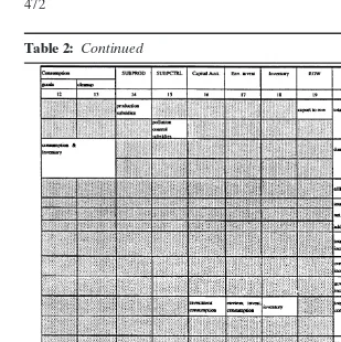
In order to capture the relevant interactions between pollution and economic activities and provide a consistent and integrated data framework for calibrating the environmental CGE model, the framework of an environmentally extended SAM (ESAM) is developed by the authors. It is presented in Table 2. The ESAM provides an integrated data system in which pollution related information, such as those concerned with pollution abatement sectors, sectoral payments for pollution cleanup, pollution emis-sion taxes, pollution control subsidies, and environmental invest-ments, are accounted for separately.
12This kind of assumption has been used by Robinson (1990).
Table 2: Framework of an Environmentally Extended Social Accounting Matrix
(Continued)
More specifically, pollution-abatement activities, i.e., the activi-ties of removing pollution, are separately listed in the activity account. The intermediate inputs of pollution-abatement sectors are presented in sub-matrix (3,2) in the commodity by activity matrix, which follows Leontief’s approach illustrated in his envi-ronmental I/O tables (1970).14Sub-matrix (2,4) in the activity by
commodity matrix presents the amount of pollutants that are abated by pollution abatement sectors. The costs for removing
Table 2: Continued
SUBPROD5subsidies to production sectors; SUBPCTRL5subsidies to pollution abatement sectors.
pollution or the payments for pollution cleanup in production sectors are presented in matrix (4,1).
production pollution are presented, together with other enterprise transfers to household, in entry (9,10).
Government efforts in pollution abatement are also reflected in government spending on pollution cleanup in entry (13,11). Household spending on pollution cleanup, if there is any, can be kept in entry (13,9). Environmental investment is separately accounted for in the environmental investment column (column 17) and row (row 17) in order to distinguish environmental invest-ment from other types of investinvest-ment and, furthermore, environ-mental investment consumption from other types of consumption. In addition, pollution generation and resource uses in physical terms are also presented in the last two columns and rows of the ESAM.
A numerical example of an ESAM using Chinese data is pre-sented in a case study in the next section. A detailed discussion of how to calibrate a CGE model to a SAM can be found in Devarajan et al. (1994).
5. CHINESE ENVIRONMENTAL POLICY ANALYSIS
5A. Country Background
Since 1978, the Chinese economy has experienced tremendous changes. From 1978 to 1993, the average growth rate of GNP was over 9 percent per annum. Besides the fast economic growth, the economy has moved significantly from a command economy toward a market-oriented economy. The number of prices con-trolled by the state, the quota of goods allocated under plans, the production share of state-owned enterprises as well as the importance of state investment financing have all dramatically dropped. The latest studies of the Chinese economy (World Bank, 1993, 1994a, 1994b) show that the market is playing a significant role in economic decision making.
Although China is telling the world a story of successful eco-nomic development, its environment is showing a very different picture. Environmental degradation now is more pervasive and serious than ever before in China. According to the 1993 Environ-mental Communique´ of China (NEPA, 1994), air pollution was serious in large and medium cities and continued to worsen in small cities.15 Among the surveyed 94 river sections running
through urban areas, 65 (69 percent) of them showed that river water was polluted. The quality of ground water became worse, and the subsidence caused by the over-exploitation of ground water occurred apparently in 36 cities. The forest coverage rate was only 12.98 percent (1989 data), and timber supply was still very tight. The soil erosion area expanded to 150 million hectare, 15.6 percent of the total land; one-third of agricultural land was faced with significant soil erosion problems; and 6.67 million hect-are of agricultural land was exposed to industrial wastes and urban refuse.
To combat environmental problems, the Chinese government has put a series of environmental policies, programs, and regula-tions in place. The major instituregula-tions and environmental policies in use include an environmental impact assessment system, an industrial pollution effluent fee system, an environmental protec-tion fund, polluprotec-tion emission permits (now on trial in some urban areas), and other environmental management measures. In 1994, the National Environmental Protection Agency of China (NEPA) launched a five-year environmental protection program, with the goals of reducing industrial pollution by treating 80 percent of all industrial waste water and 88 percent of industrial waste gases by the end of 1998.
However, due to a lack of adequate quantitative models for environmental policy analysis, the overall effectiveness of these environmental policies and programs on pollution control as well as their economic implications are still unknown. There is a need for models to assess the environmental and economic impacts of these polices and programs. Consequently, the environmental CGE model developed in Section 3 is applied to China for this purpose.
5B. The China Model
The model identifies three general types of pollution: waste water, smog dust, and solid waste.16 Thus, three corresponding
pollution-abatement sectors are included in the activity category. The model contains 289 endogenous variables in total. The exogenous or policy control variables of the model include various types of tax rates, subsidies, government expenditures, government borrowings, the average wage rate, and the foreign exchange rate.
To calibrate the environmental CGE model of China, an ESAM using Chinese 1990 data is assembled and presented in Table 3. The ESAM contains the above three types of pollution and three corresponding pollution abatement sectors. The environmental CGE model is calibrated to the ESAM.
The parameters estimated above inevitably have errors or con-tain uncercon-tainty. The errors or uncercon-tainty further affects the policy simulation results of the model. Therefore, sensitivity analy-ses are conducted to test the robustness of the simulation results to the changes in pollution intensities. Sensitivity analysis results indicate that the trends of variable changes are stable within the variation of the pollution intensities tested.17
5C. Policy-Related Findings
Using the China model, several environmental policy alterna-tives are examined. They include increasing pollution emission tax rate on waste water, subsidizing waste water treatment activities, taxing household sewage and trash, and increasing the government purchase of waste water treatment services. To assess the eco-nomic impacts of China’s five-year environmental protection pro-gram, the impact assessment of one of its major objectives, raising waste water treatment rates to 80 percent, is also conducted. Again, due to limited space, this section focuses on the impacts of alternative tax rates on waste water discharge on pollution emissions and on the Chinese economy.
China began to introduce a pollution levy system in the late 1970s. By 1990, China has set up effluent fees on the emissions of about 100 types of pollutants in four pollution categories: waste water, waste gases, solid waste, and noise. The total pollution
16Waste water and solid waste are pretty broad and vague pollution categories. The reason for selecting them was that the data of these two pollution categories are available in China’s statistical reports.
J.
Xie
and
S.
Saltzman
Table
3
:
J.
Xie
and
S.
Saltzman
Table 4: Selected Results from Pollution Emission Tax Simulations
Unit Base S1-1 S1-2 S1-3 S1-4 S1-5
Total output 100 million yuan 41806.89 41802.15 41713.91 41699.45 41687.13 41676.56
Unemployment rate percent 4.00 4.02 4.23 4.28 4.31 4.34
Price index unit less 0.9908 0.9909 0.9911 0.9911 0.9912 0.9913
Total income 100 million yuan 15928.26 15924.93 15892.49 15885.74 15880.02 15875.12
Labor Income 100 million yuan 9822.32 9820.34 9799.06 9794.82 9791.21 9788.13
Government revenue 100 million yuan 3700.98 3702.69 3690.93 3691.12 3691.24 3691.33
Government saving 100 million yuan 899.43 901.16 889.48 889.69 889.84 889.94
Investment 100 million yuan 6574.14 6574.87 6554.24 6552.52 6551.03 6549.73
Net foreign reserve 100 million yuan 683.25 682.52 679.14 678.10 677.21 676.45
Real GDP 100 million yuan 17272.14 17270.12 17227.29 17220.53 17214.77 17209.82
Percentage of industrial pollution under certain treatment to meet emission standards
Waste water percent 37.71 37.41 65.39 68.34 70.89 73.09
Smog dust percent 73.81 73.82 73.84 73.85 73.86 73.87
Solid waste percent 91.75 91.78 91.89 91.91 91.93 91.95
Total level of pollution abatement
Waste water 100 million tons 44.99 44.62 77.86 81.35 84.36 86.96
Smog dust 100 million tons 0.0599 0.0599 0.0599 0.0599 0.0599 0.0599
Solid waste 100 million tons 6.0373 6.0373 6.0373 6.0373 6.0373 6.0373
POLICY
ANALYSIS
479
Table 4: Continued
Unit Base S1-1 S1-2 S1-3 S1-4 S1-5
Total level of pollution emissions
Waste water 100 million tons 237.27 237.60 203.82 200.22 197.13 194.45
Smog dust 100 million tons 0.0308 0.0308 0.0307 0.0307 0.0307 0.0307
Solid waste 100 million tons 1.1160 1.1152 1.1043 1.1023 1.1006 1.0992
Emission tax 100 million yuan 12.02 14.45 10.41 12.14 13.56 14.76
Household waste tax 100 million yuan 0.00 0.00 0.00 0.00 0.00 0.00
Pollution subsidy 100 million yuan 0.00 0.00 0.00 0.00 0.00 0.00
Pollution compensation 100 million yuan 0.39 0.39 0.31 0.30 0.29 0.28
Utility 9.33 9.32 9.60 9.62 9.64 9.65
Note: Base5the base year simulation.
Table 5: Sectoral Changes in Output
Base S1-1 S1-2 S1-3 S1-4 S1-5
Agriculture 7659.65 7658.15 7641.90 7638.68 7635.94 7633.60 Mining 1366.90 1366.77 1364.78 1364.44 1364.14 1363.89 Light Ind. 8074.55 8072.47 8055.71 8051.90 8048.68 8045.92 Energy 1460.00 1460.80 1463.52 1463.66 1463.78 1463.88 Heavy ind. 12615.40 12614.57 12581.04 12576.42 12572.78 12569.08 Construction 3048.21 3048.90 3037.82 3037.17 3036.60 3036.10 Service 7581.20 7580.49 7569.13 7567.18 7565.52 7564.09
Unit: 100 million yuan
emission tax collected was Y 1.75 billion in 1990 and Y 2.06 billion in 1991. The pollution emission tax provides a significant source for a special environmental protection fund which mainly invests in industrial pollution control activities. Although the levy system has been praised as a successful means of raising funds for pollu-tion control, it has its weaknesses. One significant weakness is that the current fee is too low to give polluters an incentive to reduce their emissions. The need to raise the effluent fee has been discussed for years. Now the question is how much the fee should be raised and what the impact of this increase would be on the economy and pollution control.
With pollution emission tax rates incorporated into the environ-mental CGE model, one can use the model to simulate the effects of increases in pollution effluent fees. The average discharge fee on waste water is chosen for these policy experiments. The tax rate in 1990 was 0.20 yuan per ton. It is assumed arbitrarily that the government raises the tax rate incrementally by 25 percent, 50 percent, 100 percent, 150 percent, and 200 percent. Changes in key variables, such as total output, income, employment, sav-ings, price level, pollution abatement, and pollution emissions, are summarized in Table 4.
In general, as the tax rate goes up, the simulation results quanti-tatively show a steady decrease in production and a steady increase in the price index. Further, the decline in production further causes the unemployment rate to increase and the level of pollution generation to decrease. The real gross domestic product (GDP) falls as well, following the decrease in the level of production. The trends observed from the simulations agree with the pollution taxation theory of environmental economics.18
The simulation results from the model also provide more de-tailed sectoral changes in production and consumption, which allow a closer look at the impacts of pollution tax increases on each individual sector. Table 5 shows the changes in sectoral output.
With the exception of the energy sector,19 production sector
outputs drop when the tax rate on waste water discharge increase. For example, when the tax rate is raised by 50%, i.e., 0.30 yuan per ton, the output of heavy industry drops by 0.27%, or 3.44 billion yuan in absolute terms. Light industry drops by 0.23%, or 1.88 billion yuan in absolute terms. The negative impact on production is even affected in non-polluting sectors like agricul-ture (a decrease of Y 1.78 billion and 0.23%) and the service sectors (a decrease of Y 1.2 billion and 0.16%).
Concerning the effectiveness of raising the tax rate on waste water treatment, the simulations show that the scenario of raising the tax rate by 25% (from 0.25 yuan per ton in 1990 to 0.25) fails to reduce pollution emissions. As a response to the tax rate increase, the industrial sector simply goes ahead and pays more taxes for its waste water discharges. The total pollution emission tax from the three types of pollution emissions increases from Y 1.20 billion in the base year to Y 1.45 billion.
When the tax rate is raised to 0.30 yuan per ton (a 50% increase), the cleanup rate for industrial waste water rises from 37.7% (4.5 billion tons of waste water treated) in the base year to 65.4% (7.8 billion tons). Figure 5 plots the changes in the levels of waste water treatment and waste water discharge over the rise of the waste water tax rate. Note that the amount of waste water de-creases significantly after a 50% or higher increase in the waste water tax rate.
While evaluating the simulation results from environmental pol-icies, one should notice that the model only measures the economic gain or loss of an environmental policy. No non-monetary environ-mental benefits from pollution reduction have been captured by the model. However, the simulation results from this model can
Figure 5. Changes in waste water treatment and emissions.
be very useful to policy makers for evaluating the economic im-pacts and pollution reduction effects of an pollution control policy. Different from taxation, subsidy tends to result in a fall of prices and an increase in production levels of the sector receiving the subsidy. The primary results of two pollution subsidy scenarios (subsidizing waste water treatment sector by Y 200 million and Y 400 million) are shown in columns 4 and 5 (S2-1 and S2-3) of Table 6. The price of waste water cleanup falls by 10.3 percent with the low subsidy and 14.4 percent with the high subsidy. The decrease in cleanup price brings about the decrease in pollution abatement costs of the production sectors and further reduces the product prices. However, the impact on product prices is very small in both scenarios and fails to be reflected in the price index. The level of waste water treatment is driven up by the increasing demand for waste water treatment due to lower costs. The level of total waste water treatment rises by 51.7 percent (with a rise in the industrial waste water cleanup rate from 37.7 percent to 56.8 percent) when a subsidy of Y 400 million is provided for the waste water treatment sector.
Although the subsidies stimulate the production of the waste water treatment sector, they negatively affect total production output given the limited capital resources available in the econ-omy. The total output drops in both scenarios.
POLICY
ANALYSIS
483
Table 6: Selected Results from Other Environmental Policy Simulations
Unit Base S2-1 S2-2 S3 S4-1 S4-2 S5-1 S5-2
Total output 100 million yuan 41806.89 41805.95 41756.66 41780.15 41773.17 41804.29 41807.02 41761.42
Agriculture 100 million yuan 7659.65 7659.90 7651.29 7654.74 7649.23 7658.29 7659.94 7651.42
Mining 100 million yuan 1366.90 1367.00 1366.02 1366.29 1366.47 1366.92 1367.02 1366.11
Light industry 100 million yuan 8074.55 8075.03 8066.41 8069.51 8064.56 8073.21 8074.92 8066.69
Energy 100 million yuan 1460.00 1461.35 1463.23 1461.83 1462.25 1461.12 1461.23 1462.90
Heavy industry 100 million yuan 12615.40 12614.55 12595.07 12605.21 12607.29 12615.52 12615.11 12597.40
Construction 100 million yuan 3048.21 3047.04 3039.72 3044.81 3048.05 3048.84 3047.51 3041.00
Service 100 million yuan 7581.20 7581.17 7574.93 7577.76 7575.31 7580.50 7581.28 7575.49
Unemployment rate percent 4.00 4.00 4.11 4.07 4.11 4.02 4.00 4.10
Price index unit less 0.9908 0.9908 0.9908 0.9909 0.9909 0.9908 0.9908 0.9909
Total income 100 million yuan 15928.26 15929.33 15912.71 15918.48 15914.10 15926.88 15929.30 15913.62
Labor income 100 million yuan 9822.32 9822.82 9811.71 9815.90 9812.49 9821.29 9822.86 9812.41
Government revenue 100 million yuan 3700.98 3700.88 3694.21 3697.34 3703.34 3702.25 3701.64 3696.09
Government saving 100 million yuan 899.43 897.32 888.68 895.81 901.82 900.70 898.08 890.56
Investment 100 million yuan 6574.14 6572.40 6559.25 6567.83 6571.80 6574.84 6573.13 6561.33
Net foreign reserve 100 million yuan 683.25 683.72 682.37 682.24 681.39 683.01 683.32 682.26
Real GDP 100 million yuan 17272.14 17271.44 17247.26 17259.15 17253.82 17270.42 17274.04 17253.73 Percentage of industrial pollution under certain treatment to meet emission standards
Waste water percent 37.71 39.53 56.78 46.24 48.64 38.58 34.63 46.14
Smog dust percent 73.81 73.80 73.81 73.82 73.81 73.81 73.80 73.81
Solid waste percent 91.75 91.75 91.81 91.79 91.78 91.75 91.74 91.81
Price of waste water cleanup
yuan/ton 0.4107 0.3683 0.3517 0.4108 0.4108 0.4107 0.4107 0.4108
J.
Xie
and
S.
Saltzman
Table 6: Continued
Unit Base S2-1 S2-2 S3 S4-1 S4-2 S5-1 S5-2
Total level of pollution abatement
Waste water 100 million tons 44.99 47.16 67.68 55.14 58.00 46.03 46.19 64.74
Smog dust 100 million tons 0.0599 0.0599 0.0599 0.0599 0.0599 0.0599 0.0599 0.0599
Solid waste 100 million tons 6.0373 6.0373 6.0373 6.0373 6.0373 6.0373 6.0373 6.0373
Total level of pollution emissions
Waste water 100 million tons 237.27 235.11 214.30 226.96 224.05 236.21 236.08 217.26
Smog dust 100 million tons 0.0308 0.0308 0.0308 0.0308 0.0308 0.0308 0.0308 0.0308
Solid waste 100 million tons 1.1160 1.1164 1.1109 1.1127 1.1129 1.1159 1.1165 1.1114
Emission tax 100 million yuan 12.02 11.75 9.11 10.72 10.35 11.89 12.49 10.73
Household waste tax 100 million yuan 0.00 0.00 0.00 0.00 7.06 1.65 0.00 0.00
Pollution subsidy 100 million yuan 0.00 2.00 4.00 0.00 0.00 0.00 0.00 0.00
Pollution compensation 100 million yuan 0.39 0.38 0.33 0.36 0.35 0.38 0.38 0.34
Utility 9.33 9.35 9.53 9.43 9.45 9.34 9.34 9.51
Note:Base5the base year simulation.
S2-15subsidize waste water treatment sector by 200 million yuan, other control variables same as those in the base year. S2-25subsidize waste water treatment sector by 400 million yuan, other control variables same as those in the base year. S35treat 80 percent of all industrial waste water, other control variables same as those in the base year.
S4-15tax household waste water discharge by 0.2 yuan/ton, other control variables same as those in the base year. S4-25tax trash from household by 3.00 yuan/ton, other control variables same as those in the base year.
4.7 billion tons. The high subsidy scenario, however, causes pro-duction to decline more. The unemployment rate rises from 4.00 percent to 4.11 percent while income and savings fall.
Columns 4 and 5 of Table 6 also contain detailed sectoral changes in production from these two pollution subsidy simula-tions. Compared with the base year observation, one can find that subsidizing pollution abatement sectors actually hurt some less-polluting or pollution-free sectors, decreasing, for example, the outputs of the agriculture and service sectors by Y 840 million and Y 630 million, respectively. The outputs of pollution-intensive sectors like mining and energy, however, are not negatively af-fected. This is because all sectors are assumed to compete for capital resources under a tight capital supply constraint. When capital-intensive sectors, like the energy and mining sectors, be-come more cost-benefit effective due to the decrease in their pollution abatement costs, they have the advantage of gaining more capital to increase their production.
The results from other policy simulations are also presented in Table 6.
6. CONCLUDING REMARKS
Further study of this topic can take, at least, two directions: improving the model and applying the model to a broader spec-trum of policy analyses.
The model can be refined in several respects. For example, the demand of a production sector for pollution abatement services is currently specified in a simplified way. It uses average pollution cleanup rates and assumes that the unit costs for pollution abate-ment are independent of the cleanup rates. With more exploration in the economics of pollution abatement, the demand function can be more accurately defined, and the cleanup rates can be made sectorally specific. These modifications will bring the model closer to the real world case.
The pollution emission tax equation includes an implementation adjustment factor to capture the difference between the planned pollution emission taxes and the actually collected pollution emis-sion taxes. By increasing the implementation factor, one can exam-ine the outcomes of enhancing the legal enforcement of pollution emission taxes on the economy and on pollution control.
Upgrading equipment and production technology is a very effec-tive approach in reducing pollution generation and emissions. Like other countries, China has paid great attention to importing advanced and less-polluting technology from abroad to increase productivity and reduce pollution intensities. The economic and environmental impact of technological improvement can be as-sessed by changing the relevant technical coefficients such as the input-output coefficients and the pollution intensity coefficients in the model.
Although the application of the model focused on environmen-tal policy analyses, the model is also useful for analyzing the environmental impacts of an economic policy. For example, the Chinese government is planning to further increase coal produc-tion and to develop a family car industry. With an appropriate sector classification, the model could be used to assess the impacts of these policies on China’s environment.
REFERENCES
Adelman, I., and Robinson, S. (1978)Income Distribution Policy in Developing Countries: A Case Study of Korea. Stanford, CA: Stanford University Press.
Ahmad, Y.J., El Serafy, S., and Lutz, E. (1989)Environmental Accounting for Sustainable Development, A UNEP-World Bank Symposium. The World Bank.
Azis, I. (1993) Computable General Equilibrium Model for Linking Pollution and Macro-economic Variables (unpublished paper).
Bartelmus, P., Stahmer, C., and van Tongeren, J. (1993) Integrated Environmental and Economic Accounting—A Framework for an SNA Satellite System. In Toward Improved Accounting for the Environment(E. Lutz, Ed. The World Bank). Beghin, J., Roland-Holst, D., and van der Mensbrugghe, D. (1994) Trade Liberalization
and the Environment in the Pacific Basin: Coordinated Approache4s to Mexican Trade and Environmental Policy. Presented at the 1995 ASSA meeting, Washington, D.C.: January 7–9, 1995.
Bergman, L. (1988) Energy Policy Modeling: A Survey of General Equilibrium Ap-proaches.Journal of Policy Modeling10:377–399.
Bergman, L., Jorgenson, D.W., and Zalai, E. (1990a)General Equilibrium Modeling and Economic Policy Analysis. Basil: Blackwell.
Bergman, L. (1991) General Equilibrium Effects of Environmental Policy: A CGE-Model-ing Approach.Environmental and Resource Economics1: 43–61.
Bergman, L. (1993) General Equilibrium Costs and Benefits of Environmental Policies: Some Preliminary Results Based on Swedish Data. unpublished paper.
Blitzer, C., et al. (1992)Growth and Welfare Losses from Carbon Emissions Restrictions: A General Equilibrium Analysis for Egypt. Working Paper, Center for Energy Policy Research, MIT.
Boyd, R., and Uri, N.D. (1991) The Cost of Improving the Quality of the Environment. Environment and Planning A. 23:1163–1182.
Condon, T., Dahl, H., and Devarajan, S. (1986)Implementing A Computable General Equilibrium Model on GAMS: The Cameroon Model. DRD Discussion Paper. Report no. DRD290, The World Bank.
Conrad, K., and Schroder, M. (1993) Choosing Environmental Policy Instruments Using General Equilibrium Models.Journal of Policy Modeling15:521–543.
Copeland, B.R., and Taylor, M.S. (1994) North-South Trade and the Environment. Quar-terly Journal of Economics(August).
Dervis, K., de Melo, J., and Robinson, S. (1982)General Equilibrium Models for Develop-ment Policy. Cambridge: Cambridge University Press.
Devarajan, S., Lewis, J.D., and Robinson, S. (1991) From Stylied to Applied Models: Building Multisector CGE Models for Policy Analysis. (mimeo).
Devarajan, S. (1993) Can Computable General-Equilibrium Models Shed Light on the Environmental Problems of Developing Countries? unpublished paper.
Devarajan, S., Lewis, J.D., and Robinson, S. (1995) Getting the Model Right: the General Equilibrium Approach to Adjustment Policy. (mimeo).
Dowlatabadi, H., Goulder, L.H., and Kopp, R. (1994) Integrated Economic and Ecological Modeling for Public Policy Decision Making. Resources for the Future Working Paper, Washington, DC.
Dufournaud, M.C., Harrington, J., and Rogers, P. (1988) Leontief’s ‘Environmental Reper-cussions and the Economic Structure. . .’ Revisited: A General Equilibrium Formu-lation.Geographical Analysis20: 318–327.
Espinosa, J.A., and Smith, V.K. (1994)Measuring the Environmental Consequences of Trade Policy: A Non-Market CGE Analysis. presented on the 1995 ASSA meeting, Washington, D.C.: January 7–9, 1995.
Forsund, F.R., Hoel, M., and Longva, S. (1985) Production, Multi-sectoral Growth and Planning: Essays in Memory of Leif Johansen. North-Holland.
Forsund, F.R., and Strom, S. (1988)Environmental Economics and Management: Pollution and Natural Resources.London: Croon Helm.
Glomsrod, S., Vennemo, H., and Johnson, T. (1992) Stabilization of Emissions of CO2: A Computable General Equilibrium Assessment.Scandinavian Journal of Econom-ics94: 53–69.
Gruver, G., and Zeager, L. (1994) Distributional Implications of Taxing Pollution Emis-sions: A Stylized CGE Analysis. Paper presented at the Fifth International CGE Modeling Conference, October 27–29, University of Waterloo, Ontario, Canada. Hazilla, M., and Kopp, R. (1990) Social Cost of Environmental Quality Regulations: A
General Equilibrium Analysis.Journal of Political Economy98: 853–873. Idenburg, A., and Steenge, A. (1991) Environmental Policy in Single-product and Joint
Production Input-Output Models, in (F.J. Dietz, Ed.),Environmental Policy and the Economy.Amsterdam: North-Holland.
Johansen, L. (1974)A Multi-Sectoral Study of Economic Growth. 2nd, enlarged edition. North-Holland Publishing Company.
Jorgenson, D.W., and Wilcoxen, P.J. (1990) Intertemporal General Equilibrium Modeling of U.S. Environmental Regulation.Journal of Policy Modeling12: 715–744. Keuning, S. (1993) National Accounts and the Environment: the Case for a System’s
Approach. National Accounts Occasional Paper no.NA-053, Netherlands Central Bureau of Statistics.
Lee, H., and Roland-Holst, D. (1993) International Trade and the Transfer of Environmen-tal Costs and Benefits.OECD Development Centre Technical Papers,No. 91, Paris. (1993)
Leontief, W. (1970) Environmental Repercussions and the Economic Structure: An Input-Output Approach,Review of Economics and Statistics52: 262–271.
Lewis, J. (1993) Energy Pricing, Economic Distortion, and Air Pollution in Indonesia. Development Discussion Paper no. 455, Harvard Institute for International Devel-opment. Cambridge: Harvard University.
Lutz, E. (1993) Toward Improved Accounting for the Environment, An UNSTAT-World Bank Symposium. The World Bank.
Mansur, A., and Whalley, J. (1994) Numerical Specification of Applied General Equilib-rium Models: Estimation, Calibration, and Data. in Applied General EquilibEquilib-rium Analysis, (H.E. Scarf and J.B. Shoven, Eds. Cambridge: Cambridge University Press.
Nestor, D.V., and Pasurka, C.A. (1995) CGE Model of Pollution Abatement Processes for Assessing the Economic Effects of Environmental Policy.Econmic Modelling 12: 53–59.
Pearce, D.W., and Turner, R.K. (1990) Economics of Natural Resources and the Environ-ment. The Johns Hopkins University Press.
Persson, A.B. (1994). Deforestration in Costa Rica: Investigating the Impacts of Market Failures and Unwanted Side Effects of Macro Policies Using Three Different Model-ing Approaches (unpublished paper).
Piggott, J., Whalley, J., and Wigle, R. (1992) International Linkages and Carbon Reduction Initiatives. in The Greening of World Trade Issues. edited by K. Anderson and R. Blackhurst. The University of Michigan Press.
Robinson, S. (1990) Pollution, Market Failure, and Optimal Policy in an Economy-wide Framework. Working Paper no. 559, Department of Agricultural and Resource Economics. Berkeley: University of California.
Robinson, S., Subramanian, S., and Geoghegan, J. (1993) Modeling Air Pollution Abate-ment in a Market Based Incentive Framework for the Los Angeles Basin (unpub-lished paper).
Taylor, L., et al. (1979)Macro Models for Developing Countries.New York: McGraw-Hill.
Taylor, L., (1990) Structuralist CGE Models. InSocially Relevant Policy Analysis: Structur-alist Computable General Equilibrium Models for the Developing World(L. Taylor, Ed.). Cambridge, MA: The MIT Press.
United Nations. (1993b) Integrated Environmental and Economic Accounting (Interim version), Studies in Methods, Series F, 61, New York: United Nations.
Wang, Z. (1994) The Impact of Economic Integration among Taiwan, Hong Kong and China. Ph.D. Dissertation. University of Minnesota.
World Bank. (1994a)China: Internal Market Development and Regulation.Washington, DC: The World Bank.