Full Terms & Conditions of access and use can be found at
http://www.tandfonline.com/action/journalInformation?journalCode=ubes20
Download by: [Universitas Maritim Raja Ali Haji] Date: 11 January 2016, At: 19:19
Journal of Business & Economic Statistics
ISSN: 0735-0015 (Print) 1537-2707 (Online) Journal homepage: http://www.tandfonline.com/loi/ubes20
Numerically Accelerated Importance Sampling for
Nonlinear Non-Gaussian State-Space Models
Siem Jan Koopman, André Lucas & Marcel Scharth
To cite this article: Siem Jan Koopman, André Lucas & Marcel Scharth (2015) Numerically Accelerated Importance Sampling for Nonlinear Non-Gaussian State-Space Models, Journal of Business & Economic Statistics, 33:1, 114-127, DOI: 10.1080/07350015.2014.925807
To link to this article: http://dx.doi.org/10.1080/07350015.2014.925807
View supplementary material
Accepted author version posted online: 12 Jun 2014.
Submit your article to this journal
Article views: 242
View related articles
Supplementary materials for this article are available online. Please go tohttp://tandfonline.com/r/JBES
Numerically Accelerated Importance Sampling
for Nonlinear Non-Gaussian State-Space
Models
Siem Jan K
OOPMANDepartment of Econometrics, VU University Amsterdam, 1081 HV Amsterdam, The Netherlands;
Tinbergen Institute Amsterdam, The Netherlands; CREATES, Aarhus University, DK-8210 Aarhus, Denmark
Andr ´e L
UCASDepartment of Finance, VU University Amsterdam, 1081 HV Amsterdam, The Netherlands; Tinbergen Institute and Duisenberg School of Finance, 1082 MS Amsterdam, The Netherlands ([email protected])
Marcel S
CHARTHAustralian School of Business, University of New South Wales, Kensington NSW 2052, Australia
We propose a general likelihood evaluation method for nonlinear non-Gaussian state-space models using the simulation-based method of efficient importance sampling. We minimize the simulation effort by replacing some key steps of the likelihood estimation procedure by numerical integration. We refer to this method as numerically accelerated importance sampling. We show that the likelihood function for models with a high-dimensional state vector and a low-dimensional signal can be evaluated more efficiently using the new method. We report many efficiency gains in an extensive Monte Carlo study as well as in an empirical application using a stochastic volatility model for U.S. stock returns with multiple volatility factors. Supplementary materials for this article are available online.
KEY WORDS: Control variables; Efficient importance sampling; Kalman filter; Numerical integration; Simulated maximum likelihood; Simulation smoothing; Stochastic volatility model.
1. INTRODUCTION
The evaluation of an analytically intractable likelihood func-tion is a challenging task for many statistical and econometric time series models. The key challenge is the computation of a high-dimensional integral which is typically carried out by importance sampling methods. Advances in importance sam-pling over the past three decades have contributed to the in-terest in nonlinear non-Gaussian state-space models that in most cases lack a tractable likelihood expression. Examples include stochastic volatility models as in Ghysels, Harvey, and Renault (1996), stochastic conditional intensity models as in Bauwens and Hautsch (2006), non-Gaussian unobserved com-ponents time series models as in Durbin and Koopman (2000), and flexible nonlinear panel data models with unobserved het-erogeneity as in Heiss (2008).
We propose a new numerically and computationally efficient importance sampling method for nonlinear non-Gaussian state-space models. We show that a major part of the likelihood evaluation procedure can be done by fast numerical integra-tion rather than Monte Carlo integraintegra-tion only. Our main con-tribution consists of two parts. First, a numerical integration scheme is developed to construct an efficient importance den-sity that minimizes the log-variance of the simulation error. Our approach is based on the efficient importance sampling (EIS) method of Richard and Zhang (2007), which relies on Monte Carlo simulations to obtain the importance density. Second, we
propose new control variables that eliminate the first order simu-lation error in evaluating the likelihood function via importance sampling.
Numerical integration is generally highly accurate but its feasibility is limited to low-dimensional problems. Although the Monte Carlo integration method is applicable to high di-mensional problems, it is subject to simulation error. These properties are typical to applications in time series modeling. Here we adopt both methods and we show how to carry the virtues of numerical integration over to high dimensional state-space models. We depart from the numerical approaches of Kitagawa (1987) and Fridman and Harris (1998) as well as from the simulation based methods of Danielsson and Richard (1993) and Durbin and Koopman (1997). We refer to our new method
asnumerically accelerated importance sampling(NAIS).
Following Shephard and Pitt (1997) and Durbin and Koopman (1997) (referred to as SPDK), we base our importance sampling method on an approximating linear Gaussian state-space model and use computationally efficient methods for this class of mod-els. We explore two different, but numerically equivalent, sets of algorithms. The first approach follows SPDK and considers
© 2015American Statistical Association Journal of Business & Economic Statistics January 2015, Vol. 33, No. 1 DOI:10.1080/07350015.2014.925807 Color versions of one or more of the figures in the article can be found online atwww.tandfonline.com/r/jbes.
114
Kalman filtering and smoothing (KFS) methods. The second reinterprets and extends the EIS sampler in Jung, Liesenfeld, and Richard (2011) as a backward-forward simulation smooth-ing method for a linear state-space model. We clarify the rela-tions between these two methods. We further conduct a Monte Carlo and empirical study to analyze the efficiency gain of the NAIS method when applied to the stochastic volatility model as, for example, in Ghysels, Harvey, and Renault (1996). We present results for other model specifications in an online ap-pendix (supplementary materials): the stochastic duration model of Bauwens and Veredas (2004); the stochastic copula model of Hafner and Manner (2012); and the dynamic factor model for multivariate count data of Jung, Liesenfeld, and Richard (2011). The Monte Carlo study reveals three major findings. First, we show that our NAIS method can provide 40–50% reductions in simulation variance for likelihood evaluation, when compared to a standard implementation of the EIS. Second, the use of the new control variables further decreases the variance of the likelihood estimates by 20–35% relative to the use of antithetic variables as a variance reduction device. The use of antithetic variance reduction techniques may even lead to a loss of com-putational efficiency, especially for models with multiple state variables. Third, by taking the higher computational efficiency of the NAIS method into account, we find 70–95% gains in vari-ance reduction of the likelihood estimates, when compared to the standard EIS method and after we have normalized the gains in computing time. Similar improvements are obtained when we compare the EIS algorithm of Richard and Zhang (2007) with the local approximation method of SPDK.
To illustrate the NAIS method in an empirical setting, we consider a two-factor stochastic volatility model applied to time series of returns for a set of major U.S. stocks. The two-factor structure of the volatility specification makes estimation by means of importance sampling a nontrivial task. However, we are able to implement the NAIS approach using standard hard-ware and softhard-ware facilities without complications. The NAIS method reduces the computing times in this application by as much as 66% and leads to Monte Carlo standard errors for the estimated parameters which are small compared to their statisti-cal standard errors. This application illustrates that we are able to use the NAIS method effectively for estimation and inference in many practical situations of interest.
The structure of the article is as follows. Section2presents the nonlinear non-Gaussian state-space model, introduces the necessary notation, and reviews the key importance sampling methods. Our main methodological contributions are in Section
2.4and Section3, which present our numerically accelerated im-portance sampling (NAIS) method and the corresponding new control variables, respectively. Section4discusses the results of the Monte Carlo and empirical studies. Section5concludes.
2. IMPORTANCE SAMPLING FOR STATE-SPACE MODELS
2.1 Nonlinear and Non-Gaussian State-Space Model
The general ideas of importance sampling are well estab-lished and developed in the contributions of Kloek and van Dijk (1978), Ripley (1987) and Geweke (1989), among others. Danielsson and Richard (1993), Shephard and Pitt (1997) and Durbin and Koopman (1997) have explored the implementation
of importance sampling methods for the analysis of nonlinear non-Gaussian time series models. Richard and Zhang (2007) provided a short review of the literature with additional refer-ences. Our main task is to evaluate the likelihood function for the nonlinear non-Gaussian state-space model tion matrix; the dynamic properties of the stochastic vectorsyt, θt, andαt are determined by them×1 constant vectordt, the m×mtransition matrixTt, andm×mvariance matrixQt. The Gaussian innovation seriesηt is serially uncorrelated. The ini-tial mean vectora1and variance matrixP1are determined from
the unconditional properties of the state vectorαt. The system variablesZt,dt,Tt, andQtare only time-varying in a determin-istic way. The unknown fixed parameter vectorψcontains, or is a function of, the unknown coefficients associated with the observation densityp(yt|θt;ψ) and the system variables.
The nonlinear non-Gaussian state-space model as formulated in Equation (1) allows the introduction of time-varying param-eters in the density p(yt|θt;ψ). The time-varying parameters depend on the signalθt in a possibly nonlinear way. The signal vectorθt depends linearly on the state vectorαt, for which we formulate a linear dynamic model. Our general framework ac-commodates combinations of autoregressive moving average, long memory, random walk, and cyclical and seasonal dynamic processes. Harvey (1989) and Durbin and Koopman (2012) pro-vided a detailed discussion of state–space model representations and unobserved components time series models.
2.2 Likelihood Evaluation via Importance Sampling
Define andy′=(y1′, . . . , yn′),θ′=(θ1′, . . . , θn′) andα′= (α′1, . . . , αn′) . Ifp(yt|θt;ψ) is a Gaussian density with mean θt =Ztαt and covariance matrixHt, fort =1, . . . , n, Kalman filtering and smoothing methods evaluate the likelihood and compute the minimum mean squared error estimates of the state vector αt together with its mean squared error matrix. In all other cases, the likelihood for (1) is given by the analytically intractable integral (1). Kitagawa (1987) developed a numerical integration method for evaluating the likelihood integral in (2). This approach is only feasible whennis small andyt,θt, andαt are scalars.
We aim to evaluate the likelihood function by means of im-portance sampling. For this purpose, we consider the Gaussian importance density
g(α|y;ψ)=g(y|α;ψ)g(α;ψ)/g(y;ψ),
whereg(y|θ;ψ),g(α;ψ) andg(y;ψ) are all Gaussian densities and whereg(y;ψ) can be interpreted as a normalizing constant. It is implied from (1) thatg(α;ψ)≡p(α;ψ). We can express where the importance weight function is given by
ω(θ, y;ψ)=p(y|θ;ψ)/ g(y|θ;ψ). (3) We evaluate the likelihood function usingSindependent trajec-toriesθ(1), . . . , θ(S)that we sample from the signal importance The estimate (4) relies on the typically low-dimensional signal vectorθt rather than the typically high-dimensional state vector αt. Hence the computations can be implemented efficiently.
Under standard regularity conditions, the weak law of large numbers ensures that
L(y;ψ)−→p L(y;ψ), (5) whenS→ ∞. A central limit theorem is applicable only when the variance of the importance weight function exists; see Geweke (1989). The failure of this condition leads to slow and unstable convergence of the estimate. Monahan (1993) and Koopman, Shephard, and Creal (2009) developed diagnostic tests for validating the existence of the variance of the impor-tance weights based on extreme value theory. Richard and Zhang (2007) discussed more informal methods for this purpose.
2.3 Importance Density as a Linear State-Space Model
The Gaussian importance density for the state vector can be represented asg(α|y;ψ)=g(α, y;ψ)/g(y;ψ) with
where scalarat, vectorbt, and matrixCtare defined as functions of the data vectoryand the parameter vectorψ, fort =1, . . . , n. The constants a1, . . . , an are chosen such that (6) integrates to one. The set of unique importance sampling parameters is, therefore, given by
{b, C} = {b1, . . . , bn, C1, . . . , Cn}. (8)
The state transition densityg(αt|αt−1;ψ) in (6) represents the
dynamic properties ofαtand is the same as in the original model (1) becauseg(α;ψ)≡p(α;ψ). Hence, the importance density only varies with{b, C}. We discuss proposals for computing the importance parameter set{b, C}in Section2.4.
Koopman, Lit, and Nguyen (2014) show that the observation densityg(yt|θt;ψ) in (7) can be represented by a linear state-space model for the artificial observationsyt∗=Ct−1bt which are computed for a given importance parameter set {b, C}in (8). The observation equation fory∗t is given by
yt∗ =θt+εt, εt ∼N(0, Ct−1), t =1, . . . , n, (9) where θt is specified as in (1) and the innovation series εt is assumed to be serially and mutually uncorrelated with the inno-vation seriesηt in (1). The Gaussian logdensity logg(yt∗|θt;ψ)
where the constantatcollects all the terms that are not associated withθt. It follows thatat =(log|Ct| −log 2π−b′tyt∗)/2. We conclude thatg(θ, y;ψ)≡g(θ, y∗;ψ), and henceg(α, y;ψ)≡
g(α, y∗;ψ), withy∗ ′=(y∗ ′
1 , . . . , yn∗ ′).
The linear model representation allows the use of computationally efficient methods for signal extraction and sim-ulation smoothing. In particular, for the Monte Carlo evalua-tion of the likelihood as in (4), we require simulations from g(θ|y;ψ)≡g(θ|y∗;ψ) for a given set {b, C}where b andC
are functions of yand ψ. We have two options that lead to numerically equivalent results. The first option is to apply the state-space methods to model (9) as described by Durbin and Koopman (2012). Signal extraction relies on the Kalman filter smoother and simulation smoothing may rely on the methods of de Jong and Shephard (1995) or Durbin and Koopman (2002). The second option is to use a modification of the importance sampling method of Jung, Liesenfeld, and Richard (2011) which we refer to as the backward-forward (BF) method. We show in Appendix A that the approach of Jung, Liesenfeld, and Richard (2011) can be reshaped and extended to obtain a new algorithm for signal extraction and simulation smoothing applied to model (9). This completes the discussion of likelihood evaluation via importance sampling. Several devices for simulation variance reduction, including antithetic variables, can be incorporated in the computations of (4). Next we discuss a new method for choosing the importance parameter set{b, C}in (8). Existing methods are reviewed in Section2.5.
2.4 Numerically Accelerated Importance Sampling
The numerically accelerated importance sampling (NAIS) method constructs optimal values for the importance parameter set{b, C}using the same criterion for the efficient importance sampling (EIS) method of Liesenfeld and Richard (2003) and Richard and Zhang (2007). The values forb andCin the EIS
are chosen such that the variance of the log importance weights by (7). The minimization in (11) is high-dimensional and nu-merically not feasible in most cases of interest. The minimiza-tion in (11) is therefore reduced to a series of minimizations for bt andCt, for t=1, . . . , n. Hence, we obtain the importance
The NAIS method is based on the insight that the smoothing densityg(θt|y;ψ)≡g(θt|y∗;ψ) is available analytically for the
where the conditional meanθtand varianceVtare obtained from the Kalman filter and smoother (KFS) or the backward-forward (BF) smoothing method of Appendix A, in both cases applied to model (9).
This result allows us to directly minimize the low dimensional integral (13) for each time periodtvia the method of numerical integration. For most cases of practical interest, the method produces a virtually exact solution. Numerical integration is reviewed in Monahan (2001). We adopt the Gauss–Hermite quadrature method that is based on a set of M abscissae zj with associated weightsh(zj), forj =1, . . . , M. The value of
M is typically between 20 and 30. The values for the weights h(zj) are predetermined for any value ofM. The Gauss–Hermite quadrature approximation of the minimization (13) is then given by and varianceVtare defined in Equation (14) from which it fol-lows thatg( θtj|y∗;ψ)=exp(−0.5z2j)/
√
2π Vt. Further details of our numerical implementation are provided in the online ap-pendix (supplementary materials).
The minimization (15) takes place iteratively as in the original EIS method. For a given importance parameter set{b, C}, we
obtain meanθtand varianceVtfrom (14), fort=1, . . . , n. New values for bt andCt are then obtained from the minimization (15) that is reduced to a weighted least squares computation for each t. We take logp(yt|θtj;ψ) as the “dependent” vari-able, vector (1,θtj,−0.5θtj2)′as the “explanatory” variable and exp(z2j/2)h(zj)ω(θtj, yt;ψ) as the “weight” for which all terms that do not depend on zj are dropped. The regression com-putations are based on sums overj =1, . . . , M. The second and third regression estimates, those associated withθtjandθtj2, represent the new values forbt andCt, respectively. The com-putations are repeated for each tor are done in parallel. Once a new set for{b, C}is constructed, we can repeat this proce-dure. Convergence toward a final set{b, C}typically takes a few iterations.
We start the procedure by having initial values for{b, C}. A simple choice is bt =0 andCt=1, fort =1, . . . , n. We can also initialize{b, C}by the local approximation of Durbin and Koopman (1997); see Section2.5. Finally, Richard and Zhang (2007) argued that we can omit the termω( θtj, yt;ψ) for com-puting the regression “weight” without much loss of numerical efficiency. We prefer to adopt this modification because it is computationally convenient. The NAIS procedure for selecting the importance parameter set is reviewed inFigure 1.
2.5 Relation to Previous Methods
We show in Section4 that the NAIS method is an efficient method from both computational and numerical perspectives. We compare the NAIS with two related methods. The first is the local approximation method of Shephard and Pitt (1997) and Durbin and Koopman (1997) which we refer to as SPDK. It is based on a second-order Taylor expansion of logp(yt|θt;ψ) around the conditional mode ofp(θt|y;ψ) which can be com-puted iteratively using KFS or BF applied to model (9) for evaluating θt andVt as in the algorithm inFigure 1. The iter-ations require analytic expressions for the first two derivatives of logp(yt|θt;ψ), with respect toθt, fort=1, . . . , n. The con-vergence toward the mode of p(θt|y;ψ) typically takes a few iterations; see Durbin and Koopman (2012).
The second method is the efficient importance sampling (EIS) algorithm as developed by Richard and Zhang (2007). This method approximates the minimization problem in (13) via the sampling of the signalθt =Ztαtvia simulation smoothing from g(α|y;ψ), fort =1, . . . , n, rather than by numerical integra-tion as in NAIS. In the modeling framework (1), the sampling is carried out by the backward-forward sampler of Jung, Liesen-feld, and Richard (2011). The BF sampler in Appendix A is a modification and a more efficient implementation of this sam-pler. Furthermore, the introduction of antithetic variables halves the simulation effort. Koopman, Lit, and Nguyen (2014) de-velop an implementation of EIS that is based on the KFS. We emphasize that the EIS uses simulation methods both for select-ing{b, C}and for evaluating the likelihood function. In Section
4 we consider the methods of SPDK and EIS using BF and KFS. These methods for selecting the importance parameter set are reviewed in detail in the online appendix (supplementary materials).
Figure 1. NAIS algorithm for selecting the importance parameter set{b, C}.
3. NEW CONTROL VARIABLES FOR NAIS
We introduce a new set of control variables to improve the numerical efficiency of likelihood evaluation using importance sampling based on NAIS. We develop control variables that are based on specific Taylor series expansions. The control vari-ables can be evaluated by numerical integration using Gauss– Hermite quadrature. We exploit the differences between the estimates that are obtained from simulation and numerical inte-gration methods with the sole purpose of reducing the variance of importance sampling estimates. This approach of variance reduction in the context of NAIS can replace the use of the antithetic variables proposed by Ripley (1987) and Durbin and Koopman (2000).
The likelihood estimate (4) is the sample average ¯ω= S−1S
s=1ωs multiplied byg(y;ψ), where
ωs=ω(θ(s), y;ψ)= n
t=1
ωt s, ωt s=ω(θ
(s)
t , yt;ψ),
t =1, . . . , n, s=1, . . . , S,
with the importance sample weightsω(θt, yt;ψ) defined below (13),θ(s)generated from the importance densityg(θ|y;ψ), and θt(s) denoting thetth element ofθ(s), fort=1, . . . , n. The den-sityg(y;ψ) can be evaluated by the Kalman filter applied to the linear Gaussian model (9) for some value ofχ. The vari-ance of the sample average ¯ωdetermines the efficiency of the importance sampling likelihood estimate (4).
To reduce the variance of ¯ω, we construct control variates based on
x(θ, y;ψ)=logω(θ, y;ψ)=logp(y|θ;ψ)−logg(y|θ;ψ).
The tth contribution of x(θ, y;ψ) is given by x(θt, yt;ψ)= logω(θt, yt;ψ) such thatx(θ, y;ψ)=
n
t=1x(θt, yt;ψ). Given the drawsθ(1), . . . , θ(S), we define
xs =log(ωs)= n
t=1
xt s, s=1, . . . , S,
where xt s =log(ωt s), and hence ωt s =exp(xt s) for t = 1, . . . , n. We can express the sample average of ωs in terms ofxs =logωs by means of a Taylor series around some value
x, that is,
¯
ω=exp(x)1 S
S
s=1
1+[xs−x]+ 1
2[xs−x]
2
+ · · ·
.(16)
We adopt the terms involvingxt s,t =1, . . . , n, in this expan-sion as control variables. Our method consists of replacing the highest variance terms of the Taylor series by their probability limits, which we compute efficiently via the NAIS algorithm. This step clearly leads to a further reduction of the importance sampling variance and to an improvement of the numerical ef-ficiency at a low computational cost.
3.1 Construction of the First New Control Variable
We base our first control variable on the first order term (xs−x) of the Taylor series expansion (16). Under the same regularity conditions required for importance sampling, we have
¯ x = 1
S S
s=1
xs p
−→x, (17)
wherex =Egx(θ, y;ψ) and whereEg is expectation with re-spect to densityg(θ|y;ψ). The Taylor series expansion (16)
aroundx=xcan now be used to construct a first-order control
we can evaluatex by means of the Gauss–Hermite quadrature method for each time indextseparately as discussed in Section
2.4, that is,
t zj and with the numerical evaluation as in (15). The Kalman filter and smoother computesθt andVtfor t=1, . . . , n. Furthermore, we havex=nt=1xt.
The likelihood estimate (4) corrected for the first control variable is given by the importance model (9) provides an accurate approximation to the likelihood,ωsis close to one andxsis close to zero, such thatωs≈1+xs. Hence,ωs and exp(x)xs are typically highly and positively correlated. When the importance model is a less accurate approximation, the positive correlation remains, but at a more moderate level. Therefore,L(y;ψ)cis a more efficient estimate of the likelihood compared toL(y;ψ).
3.2 Construction of the Second New Control Variable
We base our second control variable on the second-order term (xs−x)2 of the Taylor series expansion (16). We aim to correct for the sample variation of (xt s−xt)2within the sample of drawsθt(1), . . . , θ
(S)
t for eachtindividually, wherextis thetth element ofx. Using the same arguments as in Section3.1, we have ¯σt2−→p σt2, where
We compute the varianceσt2using the Gauss–Hermite quadra-ture. Define
Monte Carlo and empirical evidence of the importance of the two control variables in reducing the simulation variance of the likelihood estimate obtained from the NAIS method is provided in Section4for the stochastic volatility model. More evidence for other models is presented in the online appendix (supplementary materials).
4. MONTE CARLO AND EMPIRICAL EVIDENCE FOR SV MODEL
4.1 Design of Monte Carlo Study
We consider the stochastic volatility (SV) model to illus-trate the performance of NAIS in comparison to the alternative importance sampling methods discussed in Section 2, with or without the control variables introduced in Section3. The SV model may easily be one of the most widely studied nonlinear state-space models. The references to some key developments in the SV model literature are Tauchen and Pitts (1983), Taylor (1986), and Melino and Turnbull (1990). Ghysels, Harvey, and Renault (1996) and Shephard (2005) provided detailed reviews of SV models.
For a time series of log-returnsyt, we consider thek-factor univariate stochastic volatility model of Liesenfeld and Richard (2003) and Durham (2006), that is given by
yt∼N(0, σt2), σ
2
t =exp(c+θt), θt=α1,t+ · · · +αk,t, t =1, . . . , n,
with scalar constant c, scalar signal θt andk×1 state vector αt =(α1,t, . . . , αk,t)′. The state vector is modeled by (1) with k×kdiagonal time-invariant matricesTtandQtgiven by
Tt =
φk. The signalθt represents the log-volatility.
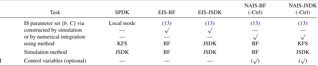
For the purpose of likelihood evaluation by importance sam-pling, we examine the performance of the SPDK method, two implementations of the standard EIS method and four imple-mentations of our NAIS method. The SPDK method is based on the mode approximation that is computed iteratively using the Kalman filter and smoother (KFS); see Section 2.5. The like-lihood function is evaluated using the simulation smoother of de Jong and Shephard (1995) or Durbin and Koopman (2002) which we refer to as JSDK. The EIS method is based on a Monte Carlo approximation to obtain the importance parameter set via the minimization (13); see Section 2.5. Our proposed NAIS method is introduced in Section2.4. The likelihood evaluation using EIS and NAIS can both be based on the JSDK simulation smoother or the BF sampler of Appendix A. Finally, both NAIS implementations can be extended with the use of the new control variables introduced in Section3.Table 1reviews the methods and their different implementations.
The design of the Monte Carlo study is as follows. We con-sider 500 random time series for each of the two SV models in
Table 1. Importance sampling methods for state-space models
NAIS-BF NAIS-JSDK
Task SPDK EIS-BF EIS-JSDK (-Ctrl) (-Ctrl)
I IS parameter set{b, C}via Local mode (13) (13) (13) (13)
constructed by simulation — √ √ — —
or by numerical integration — — — √ √
using method KFS BF JSDK BF KFS
II Simulation method JSDK BF JSDK BF JSDK
III Control variables (optional) — — — (√) (√)
NOTE: Likelihood evalution via importance sampling: I, obtain importance sampling (IS) parameter set{b, c}using methods described in Section 2.4 and 2.5; II, Sampling from the
importance density to construct likelihood function; III, in case of NIAS, with use of control variable in Section 3 or not.
our study. The first SV model has a single log-volatility compo-nent,k=1, with coefficients
c=1, φ1=0.98, ση,21 =0.0225,
which are typical values in empirical studies for daily stock returns. The second SV model hask=2 with
c=1, φ1=0.99, ση,21=0.005,
φ2 =0.9, ση,22=0.03.
We take 500 simulated time series to avoid the dependence of our conclusions on particular trajectories of the simulated states and series. For each simulated time series, we estimate the log-likelihood function at the true parameters a hundred times using different common random numbers. Hence, each cell in the tables presented below reflects 50,000 likelihood evaluations. We report the results for two different sample sizes,n=1000 andn=5000, and we useS=200 importance samples for each likelihood evaluation and for each method. The number of nodes for the numerical integration calculations is set toM=20.
We start by estimating the variance and the bias associated with each importance sampling method. We compute the re-ported statistics as the log-likelihood function for a particular method and for the jth set of common random numbers, j =1, . . . ,100, and logL(yi;ψ)=100−1 100
j=1logL
j
(yi;ψ). The true log-likelihood value is unknown but we take its “true” value as the log of the average of likelihood estimates from the NAIS method with S =200×100=20,000 importance samples. We expect the approximation error with respect to the true likelihood to be small. We compute the mean squared error (MSE) as the sum of the variance and the squared bias. The variance and the MSE are reported as a ratios with respect to the EIS-BF method; seeTable 1.
The numerical efficiency of estimation via simulation can be increased by generating additional samples. A systematic parison between methods must therefore take into account com-putational efficiency. We report the average computing times for each method on the basis of an Intel Duo Core 2.5GHz processor. We record the times required for constructing the im-portance sampling parameter set (task I) and for jointly generat-ing importance samples and computgenerat-ing the likelihood estimate (task II). In case of NAIS with control variables, we include the additional time for task III in the total time of task II. Our key summary statistic is the time normalized variance ratio of methodaagainst the benchmark methodband it is given by
Variancea/b×
where Variancea/b is the ratio of the variance defined in (18) for methodsaandband Timem
j is the time length of taskj, for j =I,II,I+II, by methodm, for m=a, b. We have excluded TimeaI from the denominator because it is a fixed cost and not
relevant for drawing additional samples.
To have the computing times of EIS and NAIS implementa-tions comparable to each other, we initialize the minimization of (11) by the local approximation for{b, C}of the SPDK method. To reduce the simulation variance for all methods, we use anti-thetic variables for location as in Durbin and Koopman (2000) except for the NAIS methods that include the control variables of Section3. We have found no evidence of importance sam-pling weights that constitute an infinite variance in our study; see the discussions in Koopman, Shephard, and Creal (2009). Our diagnostic procedure includes the verification of how sensi-tive the importance sampling weights are to artificial outliers as in Richard and Zhang (2007). We have efficiently implemented all methods using MATLAB and C.
4.2 Monte Carlo Results: Log-Likelihood Estimation
Table 2presents the results for the stochastic volatility model with k=1. The results show that our numerical integration method for constructing the importance density leads to 40%– 50% reductions in the variance of the log-likelihood estimates compared to the EIS method. In all cases the numerical gains become larger when we increase the time series dimension from n=1000 ton=5000. The use of the control variable further increases the efficiency of the NAIS method as it generates a further 20% –35% gain in producing a smaller variance. We find no deterioration in relative performance for the MSE measure,
Table 2. Log-likelihood errors for stochastic volatility model,k=1
Time step 1 Time step 2
n=1000,S=200 Variance MSE (×10) (×10) TNVAR
SPDK 12.779 12.837 0.022 0.173 5.576
EIS-BF 1.000 1.000 0.232 0.187 1.000
EIS-JSDK 1.009 1.009 0.247 0.172 1.005
NAIS-BF 0.595 0.595 0.073 0.174 0.299
NAIS-JSDK 0.594 0.594 0.070 0.175 0.297
NAIS-BF-Ctrl 0.405 0.406 0.073 0.192 0.224
NAIS-JSDK-Ctrl 0.415 0.416 0.073 0.180 0.216
Time step 1 Time step 2
n=5000,S=200 Variance MSE (×10) (×10) TNVAR
SPDK 15.025 18.594 0.052 0.908 6.152
EIS-BF 1.000 1.000 1.278 0.990 1.000
EIS-JSDK 0.997 0.998 1.246 0.908 0.885
NAIS-BF 0.503 0.501 0.364 0.928 0.245
NAIS-JSDK 0.501 0.499 0.340 0.908 0.236
NAIS-BF-Ctrl 0.380 0.381 0.418 1.002 0.206
NAIS-JSDK-Ctrl 0.375 0.376 0.398 0.939 0.189
NOTE: The table presents the numerical and computational performance of different IS methods for log-likelihood estimation. We simulate 500 different realizations from the model. For each of these realizations, we obtain log-likelihood estimates for 100 different sets of random numbers. We estimate the variance associated with each method as the average sample variance across the 500 realizations. We define the mean-square error (MSE) as the sum of the variance and the square of the average bias across the 500 realizations. We show these statistics as ratios with the standard implementation of the EIS-BF method as the benchmark. The time for step 1 column gives the fixed time cost for obtaining the parameters of the importance density, while the time for step 2 refers to the computational cost of sampling from the importance density and calculating the likelihood estimate. The TNVAR column reports
the time normalized variance ratio according to (19).Table 1lists the methods used and their acronyms. NAIS-BF-Ctrl and NAIS-JSDK-Ctrl refer to the NAIS methods with use of the
control variables of Section3. We specify the stochastic volatility model as:yt∼N(0, σt2) withσt2=exp(αt) andαt+1=0.98αt+ηtwhereηt∼N(0, ση2=0.0225) fort=1, . . . , n. confirming the accuracy of the numerical integration method for
obtaining the control variables.
The results further show that the NAIS method can also achieve substantial gains in computational efficiency. It is able to construct the importance density 70% faster than the EIS method. This result is partly due to the ability of working with the marginal densities and the scope for optimizing the computer code in this setting. In all cases the EIS method takes longer to construct the importance density than it does to generate the importance samples and to compute the log-likelihood estimate
based onS=200 simulation samples. When we normalize the variances by the length of computing time, we also obtain gains for the NAIS method.Table 2presents a total improvement of 70%–80% by the NAIS method with control variables. The gain in performance is comparable when the default EIS method is compared with the SPDK method. The results further indicate that the computing times for the BF and JSDK simulation meth-ods are equivalent for the SV model withk=1.
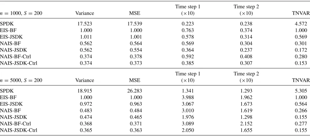
Table 3reports the findings for the SV model with two log-volatility components,k=2. These results are overall similar
Table 3. Log-likelihood errors for stochastic volatility model,k=2
Time step 1 Time step 2
n=1000,S=200 Variance MSE (×10) (×10) TNVAR
SPDK 17.523 17.539 0.223 0.238 4.572
EIS-BF 1.000 1.000 0.763 0.374 1.000
EIS-JSDK 1.011 1.001 0.578 0.314 0.569
NAIS-BF 0.562 0.564 0.569 0.304 0.301
NAIS-JSDK 0.562 0.554 0.364 0.237 0.172
NAIS-BF-Ctrl 0.374 0.378 0.592 0.408 0.280
NAIS-JSDK-Ctrl 0.374 0.373 0.385 0.307 0.153
Time step 1 Time step 2
n=5000,S=200 Variance MSE (×10) (×10) TNVAR
SPDK 18.915 26.283 1.341 1.293 5.305
EIS-BF 1.000 1.000 3.988 1.962 1.000
EIS-JSDK 0.972 0.963 3.067 1.673 0.564
NAIS-BF 0.483 0.484 3.010 1.619 0.266
NAIS-JSDK 0.474 0.465 1.976 1.298 0.155
NAIS-BF-Ctrl 0.368 0.371 3.089 2.152 0.277
NAIS-JSDK-Ctrl 0.365 0.363 2.050 1.655 0.155
NOTE: We refer to the description ofTable 2. We specify the two-factor stochastic volatility model as:yt∼N(0, σt2) withσt2=exp(αt,1+αt,2),αt+1,1=0.99αt,1+ηt,1,αt+1,1=
0.9αt,2+ηt,2, whereηt,1∼N(0, ση,21=0.005),ηt,2∼N(0, ση,22=0.03), fort=1, . . . , n.
to the ones for the SV model withk=1 inTable 2. However, we find two important differences. First, for a model with multiple states, as in the SV model withk=2, we achieve a small gain in computational efficiency by switching from the BF sampler to the JSDK sampler. The main reason is that JSDK is able to simulate the univariate signalθtdirectly whereas the BF sampler needs to simulate the signal via the (multiple) state vectorαt. Hence, we obtain around 83% reductions in the variance nor-malized by time when using the NAIS-JSDK method instead of the EIS-BF method.
The second difference between the results for the SV model withk=1 andk=2 concerns the variance reduction that we obtain by using control variables in the likelihood estimation. For the case of k=2, the variance reductions due to the control variables are similar to those fork=1, but the relative increase in the computational cost for step 2 is higher. This is because antithetic variables reduce the computational effort for simulation.
4.3 Parameter Estimation for the SV Model Using NAIS
To illustrate the performance of our proposed NAIS method in more detail, we consider the simulated maximum likelihood estimation of the unknown parameters in a multifactor stochastic volatility model. We report our findings from both a Monte Carlo study and an empirical study below. We carry out parameter estimation using the following consecutive steps:
1. Set a starting value for the estimate of parameter vectorψ.
2. Set starting values for the importance sampling parameterχ in (8).
3. Maximize the log-likelihood function with respect toψusing the NAIS-JSDK method withS=0 and only the first control variate; use the estimates as starting values for the next step. 4. Maximize the log-likelihood function with respect toψusing
the NAIS-JSDK-Ctrl method withS >0.
The estimation in Step 3 concerns an approximate log-likelihood function. It is fast and requires no simulation, only numerical integration. The computational efficiency of this pro-cedure is primarily due to the accurate approximation of the log-likelihood function calculated by the NAIS-JSDK method withS=0 and the first control variate from Section3. As a re-sult, the convergence of the maximization in the last step is fast as it only requires a small number of iterations. The consequence is that we can setSat a high value in Step 4 as it only marginally increases the required computing time. The maximizations in Steps 3 and 4 are based on a quasi-Newton method. The use of common random numbers in Step 4 for each likelihood estimation leads to a smooth likelihood function inψ, which is necessary for the application of the quasi-Newton opti-mization methods. In both studies below we set S=200 in Step 4.
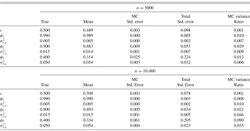
4.3.1 Monte Carlo Evidence. We consider the k-factor
stochastic volatility model withk=3 for time series of lengths n=5000 and n=10,000. The true parameter values are set to d =0.5, φ1=0.99, φ2=0.9, φ3=0.4, ση,21=0.005,
σ2
η,2=0.016, andσ 2
η,3=0.05. We take these parameter values
also as the starting values for parameter estimation. We draw 100
Table 4. Parameter estimation for stochastic volatility model,k=3
n=5000
MC Total MC variance
True Mean Std. error Std. error Ratio
c 0.500 0.489 0.003 0.098 0.001
φ1 0.990 0.989 0.000 0.005 0.010
σ2
1,η 0.005 0.005 0.000 0.002 0.007
φ2 0.900 0.883 0.009 0.055 0.029
σ2
2,η 0.015 0.014 0.001 0.007 0.009
φ3 0.400 0.314 0.025 0.224 0.012
σ2
3,η 0.050 0.054 0.003 0.032 0.006
n=10,000
MC Total MC variance
True Mean Std. Error Std. Error Ratio
c 0.500 0.500 0.003 0.078 0.001
φ1 0.990 0.990 0.000 0.003 0.008
σ2
1,η 0.005 0.005 0.000 0.002 0.010
φ2 0.900 0.893 0.005 0.034 0.021
σ2
2,η 0.015 0.015 0.001 0.005 0.046
φ3 0.400 0.334 0.061 0.205 0.090
σ2
3,η 0.050 0.054 0.004 0.023 0.035
NOTE: We simulate 100 trajectories of a three-factor stochastic volatility model. For each of these realizations, we obtain 20 simulated maximum likelihood parameter estimates based on different sets of common random numbers and using the NAIS-JSDK method. We first show the average parameter estimates across the 500 replications. The Monte Carlo (MC) standard error column reports the square root of the average of the sample variance of the parameter estimates across the 100 realizations. The total standard error column shows the square-root of the sum of the MC variance and the variance of the average estimates across the 100 trajectories. Finally, we obtain the MC variance ratio by dividing the MC variance by
the total variance. The starting values are the true parameters. The average computing time was 65s and 123s forn=5000 andn=10,000,respectively.yt∼N(0, σt2),t=1, . . . , n,
σ2
t =exp(θt),θt=d+α1,t+α2,t+α3,t,αt=T αt−1+ηt,α1∼N(a1, P1),ηt∼N(0, Q), whereTis a diagonal matrix with elementsφ1,φ2, andφ3andQis a diagonal matrix with
elementsσ2
η,1,ση,22, andση,23.
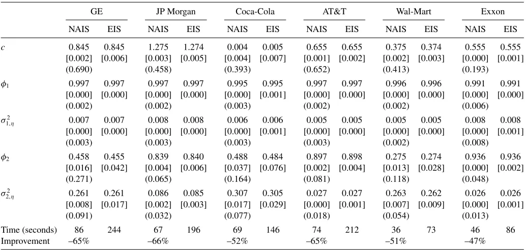
Table 5. Two-factor stochastic volatility model: Empirical study
GE JP Morgan Coca-Cola AT&T Wal-Mart Exxon
NAIS EIS NAIS EIS NAIS EIS NAIS EIS NAIS EIS NAIS EIS
c 0.845 0.845 1.275 1.274 0.004 0.005 0.655 0.655 0.375 0.374 0.555 0.555
[0.002] [0.006] [0.003] [0.005] [0.004] [0.007] [0.001] [0.002] [0.002] [0.003] [0.000] [0.001]
(0.690) (0.458) (0.393) (0.652) (0.413) (0.193)
φ1 0.997 0.997 0.997 0.997 0.995 0.995 0.997 0.997 0.996 0.996 0.991 0.991
[0.000] [0.000] [0.000] [0.000] [0.000] [0.001] [0.000] [0.000] [0.000] [0.000] [0.000] [0.000]
(0.002) (0.002) (0.003) (0.002) (0.002) (0.006)
σ2
1,η 0.007 0.007 0.008 0.008 0.006 0.006 0.005 0.005 0.005 0.005 0.008 0.008
[0.000] [0.000] [0.000] [0.000] [0.000] [0.001] [0.000] [0.000] [0.000] [0.000] [0.000] [0.001]
(0.003) (0.003) (0.003) (0.003) (0.002) (0.008)
φ2 0.458 0.455 0.839 0.840 0.488 0.484 0.897 0.898 0.275 0.274 0.936 0.936
[0.016] [0.042] [0.004] [0.006] [0.037] [0.076] [0.002] [0.004] [0.013] [0.028] [0.000] [0.002]
(0.271) (0.065) (0.164) (0.081) (0.118) (0.048)
σ2
2,η 0.261 0.261 0.086 0.085 0.307 0.305 0.027 0.027 0.263 0.262 0.026 0.026
[0.008] [0.017] [0.002] [0.003] [0.017] [0.029] [0.000] [0.001] [0.007] [0.009] [0.000] [0.001]
(0.091) (0.032) (0.077) (0.018) (0.054) (0.013)
Time (seconds) 86 244 67 196 69 146 74 212 36 73 46 86
Improvement –65% –66% –52% –65% –51% –47%
NOTE: We estimate a two-component stochastic volatility specification for the daily returns of six Dow Jones index stocks in the period between January 2001 and December 2010 (2512 observations). We repeat the NAIS-JSDK and EIS-BF estimation methods a hundred times with different random numbers. The Monte Carlo and statistical standard errors are in brackets [ ] and parentheses ( ), respectively. We specify the model asyt∼N(0, σt2),t=1, . . . , n,σt2=exp(θt),θt=c+α1,t+α2,t,αt=T αt−1+ηt,α1∼N(a1, P1),ηt∼N(0, Q), whereT
is a diagonal matrix with elementsφ1, andφ2andQis a diagonal matrix with elementsση,21, andση,22.
different time series. For each realized time series, we obtain 20 parameter estimates under different sets of common numbers and compute the Monte Carlo variance. We report the Monte Carlo standard error as the square root of the average sample variance across the 100 realizations. Since we set the true param-eters ourselves, we also calculate the mean square error (MSE) of the estimates. It allows us to directly compare the relative importance of the simulation and statistical errors in estimating the parameters.
Table 4 summarizes the results. The average computing time for estimation is 65 and 123 seconds forn=5000 and n=10,000, respectively. We learn from Table 4that despite the complexity of the model and the large sample sizes, the sim-ulation errors in parameter estimates are small both in absolute and in relative terms. Forn=5000 (n=10,000), the Monte Carlo variances represent between 0.1% (0.1%) and 3% (9%) of the total MSEs. Except for the autoregressive coefficient φ3, we observe no relevant deterioration in the Monte Carlo
variances for the case in whichn=10,000. It emphasises the effectiveness of the NAIS-JSDK method for high-dimensional problems.
4.3.2 Empirical Evidence. We investigate whether the
NAIS method extends its Monte Carlo performance to real data.
Table 5reports the estimation of a two-component stochastic volatility specification for the daily returns of six Dow Jones index stocks in the period between January 2001 and December 2010. The sample covers 2512 observations. We repeat the es-timation process for each series a hundred times with different random numbers.
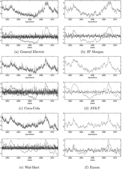
The empirical results confirm the Monte Carlo results for parameter estimation. For example, the simulation errors in pa-rameter estimates are negligible for persistent state processes, that is, for autoregressive coefficients larger than 0.9. For three of the stocks, parameter estimation has been more challeng-ing because the second volatility factor is weakly persistent and noisy. The Monte Carlo variances of the parameters correspond-ing to the second factor are approximately 5% of the statistical variance. However, the relatively low estimation times (between 46 and 86 sec) indicate that we can consider larger importance samples, which enable us to better identify the second volatility component. Figure 2 presents the signal and factor estimates based on parameter estimates fromTable 5.
Table 6. Variance reductions in parameter estimation
GE JPM KO T WMT XOM
c 0.127 0.482 0.293 0.482 0.160 0.559
φ1 0.057 0.068 0.089 0.068 0.066 0.109
σ2
1,η 0.051 0.052 0.090 0.052 0.042 0.118
φ2 0.148 0.408 0.237 0.408 0.184 0.216
σ2
2,η 0.207 0.492 0.324 0.492 0.266 0.629
NOTE: The table presents the ratios between the Monte Carlo variances of the NAIS-JSDK method against the EIS-BF method inTable 4.
Figure 2. Estimated log-variance (top) and states (bottom) for six Dow Jones stocks.
Table 5also presents the estimated parameters obtained from the EIS-BF method. The estimates obtained from the two meth-ods are identical for almost all parameters. The computation times, however, are not the same.Table 6reports ratios between the Monte Carlo variances of the estimated parameters obtained from the NAIS-JSDK and EIS-BF methods. We again find that the NAIS-JSDK method leads to substantial relative gains in numerical efficiency. However the differences have only
prac-tical relevance for persistent state variables. Substantial reduc-tions in computing time are also achieved by the NAIS-JSDK algorithm.
4.4 Further Evidence for Other Models
We have extended the Monte Carlo study for the SV model as reported above for a range of other dynamic models,
including the stochastic conditional duration model of Bauwens and Veredas (2004), the stochastic copula model of Hafner and Manner (2012) and the dynamic one-factor model for multi-variate Poisson counts of Jung, Liesenfeld, and Richard (2011). All of these models can be readily handled by the importance methods proposed in this article. As the main findings do not deviate substantially from the ones reported for the SV model, we provide the Monte Carlo results for these additional models in the online appendix (supplementary materials).
5. CONCLUSION
We have developed a new efficient importance sampling method for the evaluation of the likelihood function of nonlinear non-Gaussian state-space models. The numerically accelerated importance sampling (NAIS) approach is a nontrivial mix of nu-merical and Monte Carlo integration methods. We use Gauss– Hermite quadratures for constructing the importance sampler. The Monte Carlo evaluation of the likelihood function is pri-marily based on Kalman filtering and smoothing methods. We introduce new control variables to further reduce the sampling variance of the Monte Carlo estimate of the likelihood function. We have carried out a comprehensive simulation study to verify the performance of our approach relative to other importance sampling methods for a variety of financial time series models. Our empirical application to U.S. stock returns shows that the NAIS method produces reliable results in a numerically and computationally efficient way.
APPENDIX A: BACKWARD-FORWARD (BF) SMOOTHING AND SIMULATION
We present new smoothing and simulation smoothing algorithms that can be regarded as alternatives to the Kalman filter smoother (KFS) and to the JSDK simulation smoother, respectively. The new algorithms directly stem from the Gaussian EIS sampler developed by Jung, Liesenfeld, and Richard (2011). We propose a more efficient for-mulation, extend it to the more general model (1) and we show how it can be used for computing the smoothed estimates of the state vector. The algorithms are numerically equivalent to the KFS and JSDK, but their computational efficiencies can be different.
We derive the backward-forward (BF) method using the importance model given by (6) and (7). We suppress the dependence of all densities on the parameter vectorψ. The sampler is based on the following decomposition:
state vector transition density as implied by (1), and the functionsχt(·)
andζt(·) are chosen such thatg(αt|αt−1, y), the individual importance
density at timet, integrates to one. For the functionχt(αt−1, bt, Ct),
this is accomplished by argumentsbtandCt. The function
ζt(αt, bt+1, Ct+1)∝1/ χt+1(αt, bt+1, Ct+1) (A.1)
counters the integration constant for the next periodt+1. Hence, functionζt(·) is of key importance in the backward-forward sampler as
it implies that
represents the smoothing density g(α|y) in the same way the KFS applied to the approximating linear state-space model (9) represents
g(α|y).
Constructing the sampler:We follow Jung, Liesenfeld, and Richard (2011) by adopting an induction argument and defining the integration constant as
where scalarrt, vectorqt and matrixPt have closed form expressions
as functions of parameter vectorψ and the importance parametersbt
and Ct, but do not depend on the state vectors, for example,Pt=
which is a Gaussian kernel as well. The normal distribution with the canonical form exp(δtαt−α′ttαt/2) has mean vectorµt =−t1δtand
variance matrixt=−t1form×1 vectorδt andm×msymmetric
positive definite (precision) matrixt. After some minor manipulation,
we can show that the mean vector and variance matrix ofg(αt|αt−1, y)
are given by
µt =t(Z′tbt+Q−t−11(dt−1+Tt−1αt−1)+qt+1),
t =(Q−t−11+Z′tCtZt+Pt+1)−1, (A.6)
respectively. Given the expressions for the meanµt and the variance
t, it follows immediately thatg(αt|αt−1, y) can be represented by the
Equation (A.7) forαt suggests a forward recursion to simulate from
g(αt|y). The implementation is simple and computationally efficient
using this construction.
Backward pass:Next, we need to show that (A.3) holds and how the integration constantχt(·) is computed. In particular, we require an
expression for rt in (A.3) for the actual calculation ofg(αt|αt−1, y)
which is needed to compute the importance weights. The functionχt(·)
is given by the integration constant for a Gaussian kernel with meanµt
and variancet divided by the terms ing(αt|αt−1) that do not depend
onαt:
By substitutingµtof (A.6) into (A.8) and after some manipulation, we
obtainχt(·) in the form of (A.3) with
with t defined in (A.6), thus completing the induction argument.
We evaluatert,qt, andPt by a backward recursion that we initialize
withζn(·)=1. It implies that we can initialize the recursion (A.9) by
qn+1=0 andPn+1=0.
Simulation smoothing (forward pass): For a given set of impor-tance parameters, we determineg(αt|αt−1, y) by the backward
recur-sion (A.9); the order of computations aret, Pt,qt, andrt. We use
d∗
t−1,Tt∗−1andt computed during the backward pass for simulating
fromg(α|y) by means of the forward pass (A.7).
Evaluation of likelihood function for the importance density model:
The simulated likelihood estimate is given by (4) where it follows from the results above that
State smoothing (forward pass): For the implementation of the NAIS method using the backward-forward method, we require the smoothed estimate ofθt =Ztαt from the Gaussian importance
den-sityg(αt|y). We obtain the smoothed meanαt =E(αt|y) and variance
The document with supplementary material consists of three parts. The first part provides a basic review of the numerical integration method that is relevant for our use in the context of determining the importance sampling parameters. The second part presents detailed al-gorithmic descriptions of the three importance sampling methods that we discuss and compare in the main paper : the SPDK, the EIS and the NAIS methods. All calculations in our paper are based on the imple-mentations as described in detail here. The third part contains further results of our extended Monte Carlo study. In particular, we present the same Monte Carlo results as for the stochastic volatility model in the main article but now for the stochastic conditional duration model, the stochastic copula model, and the dynamic factor model for pois-son counts. These results are for a single element state vector in the first two cases and for a multiple dimensional state vector in the latter case.
ACKNOWLEDGMENTS
The authors thank the seminar participants at the University of Mannheim, TI Amsterdam, Chicago Booth School of Business, Uni-versit´e Paris I, Sorbonne, and the 4th CSDA conference in London, for their insightful comments. S.J. Koopman acknowledges the sup-port from CREATES, Center for Research in Econometric Analysis of Time Series (DNRF78), funded by the Danish National Research Foun-dation. A. Lucas acknowledges the financial support of the Dutch Na-tional Science Foundation (NWO, grant VICI453-09-005). M. Scharth acknowledges partial support from the Australian Research Council grant DP0667069.
[Received January 2012. Revised March 2014.]
REFERENCES
Bauwens, L., and Hautsch, N. (2006), “Stochastic Conditional Intensity Pro-cesses,”Journal of Financial Econometrics, 4, 450–493. [114]
Bauwens, L., and Veredas, D. (2004), “The Stochastic Conditional Duration Model: A Latent Factor Model for the Analysis of Financial Durations,”
Journal of Econometrics, 119, 381–412. [115,125]
Danielsson, J., and Richard, J. F. (1993), “Accelerated Gaussian Importance Sampler With Application to Dynamic Latent Variable Models,”Journal of Applied Econometrics, 8, 153–174. [114,115]
de Jong, P., and Shephard, N. (1995), “The Simulation Smoother for Time Series Models,”Biometrika, 82, 339–350. [116,119]
Durbin, J., and Koopman, S. J. (1997), “Monte Carlo Maximum Likeli-hood Estimation for Non-Gaussian State-Space Models,”Biometrika, 84, 669–684. [114,115,117]
——— (2000), “Time Series Analysis of Non-Gaussian Observations Based on State-Space Models From Both Classical and Bayesian Perspectives,”
Journal of the Royal Statistical Society, Series B, 62 3–56. [114,118,120] ——— (2002), “A Simple and Efficient Simulation Smoother for State-Space
Time Series Analysis,”Biometrika, 89, 603–616. [116,119]
——— (2012),Time Series Analysis by State-Space Methods(2nd ed.), Oxford: Oxford University Press. [115,116,117]
Durham, G. B. (2006, July), “Monte Carlo Methods for Estimating, Smoothing, and Filtering One- and Two-Factor Stochastic Volatility Models,”Journal of Econometrics, 133, 273–305. [119]
Fridman, M., and Harris, L. (1998), “A Maximum Likelihood Approach for Non-Gaussian Stochastic Volatility Models,”Journal of Business and Eco-nomic Statistics, 16, 284–291. [114]
Geweke, J. (1989), “Bayesian Inference in Econometric Models Using Monte Carlo Integration,”Econometrica, 57, 1317–1739. [115,116]
Ghysels, E., Harvey, A. C., and Renault, E. (1996), “Stochastic Volatility,” in
Handbook of Statistics(Vol. 14) eds. G. Maddala and C. Rao, Amsterdam: Elsevier. [114,119]
Hafner, C., and Manner, H. (2012), “Dynamic Stochastic Copula Models: Esti-mation, Inference and Applications,”Journal of Applied Econometrics, 27, 269–295. [115,125]
Harvey, A. C. (1989), Forecasting, Structural Time Series Models and the Kalman Filter, Cambridge: Cambridge University Press. [115]
Heiss, F. (2008), “Sequential Numerical Integration in Nonlinear State-Space Models for Microeconometric Panel Data,”Journal of Applied Economet-rics, 23, 373–389. [114]
Jung, R., Liesenfeld, R., and Richard, J. F. (2011), “Dynamic Factor Mod-els for Multivariate Count Data: An Application to Stock-Market Trad-ing Activity,”Journal of Business and Economic Statistics, 29, 73–85. [115,116,117,125]
Kitagawa, G. (1987), “Non-Gaussian State-Space Modeling of Nonstation-ary Time Series,” Journal of the American Statistical Association, 82, 1032–1063. [114,115]
Kloek, T., and van Dijk, H. K. (1978), “Bayesian Estimation of Equation System Parameters: An Application by Monte Carlo,” Econometrica 47, 1–20. [115]
Koopman, S. J., Lit, R., and Nguyen, T. M. (2014), “Modified Efficient Im-portance Sampling for State-Space Models With an Application,” working paper #1427, Department of Econometrics, VU University, Amsterdam. [116,117]
Koopman, S. J., Shephard, N., and Creal, D. (2009), “Testing the Assump-tions Behind Importance Sampling,”Journal of Econometrics, 149, 2–11. [116,120]
Liesenfeld, R., and Richard, J. F. (2003), “Univariate and Multivariate Stochas-tic Volatility Models: Estimation and DiagnosStochas-tics,”Journal of Empirical Finance, 10, 505–531. [116,119]
Melino, A., and Turnbull, S. (1990), “Pricing Foreign Currency Options With Stochastic Volatility,”Journal of Econometrics, 45, 239–265. [119] Monahan, J. F. (1993), “Testing the Behaviour of Importance Sampling
Weights,”Computer Science and Statistics: Proceedings of the 25th An-nual Symposium on the Interface, 112–117. [116]
——— (2001),Numerical Methods of Statistics, Cambridge: Cambridge Uni-versity Press. [117]
Richard, J. F., and Zhang, W. (2007), “Efficient High-Dimensional Importance Sampling,” Journal of Econometrics, 141, 1385–1411. [114,115,116,117,120]
Ripley, B. D. (1987),Stochastic Simulation, New York: Wiley. [115,118] Shephard, N. (2005),Stochastic Volatility: Selected Readings, Oxford: Oxford
University Press. [119]
Shephard, N., and Pitt, M. (1997), “Likelihood Analysis of Non-Gaussian Mea-surement Time Series,”Biometrika, 84, 653–667. [114,115,117]
Tauchen, G., and Pitts, M. (1983), “The Price Variability-Volume Relationship in Speculative Markets,”Econometrica, 51, 485–505. [119]
Taylor, S. J. (1986),Modelling Financial Time Series, Chichester, UK: Wiley. [119]