Optimal Factor-Level Condition in Parameter Design by Using
Static SN Ratio
Kenzou Hanada
a, Hiroshi Morita
a*a
Department of Information and Physical Sciences, Osaka University, Japan Accepted October 2007
Available online
Abstract
In recent years, SN ratio has come into use in areas of design and development. It is desirable as the SN ratio is defined to find the solution with the smallest scatter. However, it can not be applied to every case. In design of parameters by Taguchi method, decision based on the SN ratio may cause some problems. Observation of experiment varies due to the sampling error even if it is sampled from the same population. And the SN ratio calculated from samples varies, too. When judged only by the SN ratio of the experiment result, it has the danger to end up unacceptable as the desired optimal condition. The failure to locate the optimal condition can be prevented when the amount of influence to the SN ratio by sampling error is estimated quantitatively. We analyze the characteristics of the behavior of SN ratio, and propose an improved procedure to determine the optimal parameters.
Keywords:SN ratio; Taguchi’s terminology; Static characteristics
1. Introduction*
Recently, Quality Engineering (Taguchi Method) is widely applied to the research and development of many types of industries with the purpose of obtaining robust design. Taguchi Method is being made use of especially in the process of product development. As the result, many achievements are announced in the quality engineering conferences.
The other method having been used in the R&D field is the design of experiment method. This method uses the actually measured physical values and uses them as the evaluation index (characteristic values) to perform statistic judgment. Analysis of variance is usually applied where the variation of average of each characteristic value is used in comparison with the error to determine its effect. In other words, the population mean of characteristic value in interest is mainly discussed in this design of experiment method.
As for this quality engineering, the evaluation is not made by the quality character actually measured, but by using the substitution characteristic value of the SN ratio calculated from more than one quality characteristic values. It is said that by using this SN ratio, both the average and dispersion in the tested condition can be evaluated at the same time.
*
Corresponding author. E-mail: morita@ist.osaka-u.ac.jp
Many successful examples are reported; however, considerable numbers of failures are also reported. There has been little research made on these causes. Therefore, there are not few voices from the industrial world requesting to clarify the causes of failures.
On the other hand, more than one characteristic values are used in the parameter design in quality engineering for each combination of factor levels, and the SN ratio is obtained from the dispersion information. An error factor is introduced to each of these characteristic values to cause conditional change. At this time, orthogonal array is used. The combination of factor-levels providing the largest SN ratio is considered the most suitable in quality engineering at the first step. The population mean of the characteristic value is adjusted to the desired value at the next step. These are the characteristics of this parameter design. It is usual to perform a confirmation experiment of the most suitable case, as this method is not a complete block design.
2. Troubles in Experiments Using Static SN Ratio
2.1 Example of Confusing Numerical Values
In order to clarify the problem in the nominal-the- best type character, three leveled one-dimensional array with three time repetitions is used here. The higher the SN ratio is, the better the solution is. Three factor-level conditions are as follows:
A1: Basic condition
Table 1. Result of the1st-step Experiment
Step-1 A1 A2 A3
1 3 5 2
2 5 7 3 Data
3 7 9 4
Mean m 5.0 7.0 3.0
Standard deviation
σ 2.00 2.00 1.00
/
m σ 2.5 3.5 3
2
( / )m σ 6.25 12.25 9
SN-ratio 7.96 10.88 9.54
Rank (SN-ratio) 3 1 2
Sensitivity 13.98 16.90 9.54
Rank (sensitivity) 2 1 3
Table 2. Result of the 2nd-Step Experiment
Step-2 A1 A2 A3
1 13 15 12
2 15 17 13 Data
3 17 19 14
Mean m 15.0 17.0 13.0
Standard deviation
σ 2.00 2.00 1.00
/
m σ 7.5 8.5 13
2
( / )m σ 56.25 72.25 169
SN-ratio 17.50 18.59 22.28
Rank (SN-ratio) 3 2 1
Sensitivity 23.52 24.61 22.28
Rank (sensitivity) 2 1 3
A2: High-mean condition (larger mean and same dispersion)
A3: Low-dispersion condition (same mean and smaller dispersion with half the standard-deviation)
The target of the mean value is assumed to be 17.0. At Step-1, we calculate the SN ratio as shown in Table 1. The preferred order of cases is as A2 (10.88: best), A3 (9.54) and A1 (7.96: worst). The highest SN ratio is obtained by the largest mean value case. The smaller dispersion case follows. But, the mean value does not reach 17.0 as desired.
In Step-2, the mean is increased by 10 using a control element as the basic condition (A2 with the mean of 7.0) is judged the best in Step-1. The results are shown in the Table 2. (The A2 case in Step-2, however, is judged to be good)
In Step-2, the ranking has changed to the order of A3 (22.28: best), A2 (18.59) and A1 (17.50: worst). It contradicts with the result of Step-1. (The first and second preferences have turned over.) Without the knowledge of the phenomenon pointed out here, the A3 case is discarded in Step-1 and fails to be adopted in Step-2.
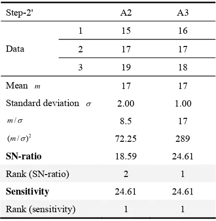
In order to clarify the issue, the mean values of both cases are made identical. The modified cases and their results are shown below (the mean of A2 and A3 are 17.0) in Table 3. When order is judged by the obtained SN ratio, the result is A3 (Good) to A2 (Bad).
Table 3. Modification of the Mean Value of the 2nd-step
Step-2' A2 A3
1 15 16
2 17 17 Data
3 19 18
Mean m 17 17
Standard deviation σ 2.00 1.00
/
m σ 8.5 17
2
(m/ )σ 72.25 289
SN-ratio 18.59 24.61
Rank (SN-ratio) 2 1
Sensitivity 24.61 24.61
Rank (sensitivity) 1 1
Note: The mean of the A3 and A2 factor levels are made identical. It is the same as the result of Step-2. The difference in calculated SN ratio becomes much bigger. Of course, sensitivity becomes the same from its definition, and it does not work as an evaluation measure at this phase.
In the general practice of the quality engineering, the condition giving the biggest SN ratio (the condition of the smallest dispersion) is looked for in Step-1. Then the mean is modified by using the sensitivity information in the next Step-2. In case there is no condition providing the desired target value at Step-1, as described above, A2 case is evaluated as the best and A3 becomes the third as long as the case closest to the target value is considered the best according to the sensitivity. This undesirable result is caused by the sole dependence to the mean value and standard deviation in Step-1 and Step-2, respectively.
It is well known that the observation value does not always become the same even if it is sampled from population of the same mean value and standard deviation. When the mean value is changed, the SN ratios are also changed for the nominal-the-best type character, the larger-the-better type character, and the smaller-the- better type character. It has the danger that the selected optimal condition combination is sometimes mistaken.
When A3 condition is removed from the candidate at Step-1, the optimal condition is lost or overlooked eternally in the actual development of new product. The parameter design proposes to find the condition providing the least dispersion at Step-1, and to modify the mean value at Step-2. The present definition is not appropriate, because the condition of the minimum dispersion is not evaluated as the best condition at Step-1. If only the dispersion of every treatment is to be evaluated, it is not necessary to calculate it again.
2 2 2
2
(Dispersion in the treatment) (sensitivity) (SN-ratio)
log log( / )
As shown above, the dispersion of every treatment is obtained by deducting the SN ratio from the sensitivity, and it is possible to evaluate by this value. Note that it becomes negative when the standard deviation σ<1, and it becomes positive when σ >1. As long as these conditions are met, the optimal case is identified by finding the condition providing the least dispersion at Step-1. It is no longer necessary to get into Step-2.
If the true mean value is known, the mean values can be modified to be identical. Then the SN ratio can be compared to identify the optimal case as shown in Table 3. Step-2 is no longer needed and the efficiency of the experiment improves drastically. Therefore, it is a must to make it always possible to select a case whose mean value is close enough to the target.
3. Characteristics of SN Ratio
Characteristic value to be used to calculate a SN ratio is considered to have the normal distribution. The test method based on the non-central t distribution proposed by Nagata, Miyagawa, and Yokozawat (2003) is derived from this. They propose a test method on dynamic character of SN ratio. Miyagawa (2006) also prescribes convex enclosed territory of the standard deviation σ and the mean μ , and explains the maximum SN ratio problem. In reality, μ σ/ giving the maximum SN ratio is not known beforehand. If it is already known, it is not needed to search it by the experiment. If the desired μ σ/ is already known, the SN ratio is obtained by calculation. We have only to confirm if it is true by experiment, only with one factor level of combination. The problem is that it is not clear whether the average and dispersion obtained in the experiment show the genuine mean and standard deviation. On the other hand, in daily experiment practice, the obtained candidate is taken as optimal without any doubt, and the confirmation experiment is carried out, in most cases, only for this single condition. A few prudent people run the confirmation experiment also for the second (and third) combinations. At this time, there is no clear criterion to what extent the confirmation experiment coverage should be extended, and the person in charge of the experiment decides it arbitrarily.
We propose a new method for this judgment procedure. As described before, regard the characteristic value to have the normal distribution. What we are searching is the true value. Therefore, you have only to find the expected value from the value obtained by the experiment. The definition of SN ratio tells that the mean μ and standard deviation σ of the characteristic value have some influence to the true value. When the characteristic value has the normal distribution, it is well known that the mean μ and dispersion σ2
follow t -distribution and
2
χ -distribution, respectively.
The definition of SN ratio contains both the average and dispersion term of the data. The average of sample follows normal distribution (u) and the dispersion of sample follows χ2
-distribution (χ2
). The average and dispersion of samples are independent [3]. The above is clear from the conventional mathematical statistics theory. Then, the probability density functions of the average and dispersion of sample are shown in the following equations with the definition of
( )/
2
Moreover, by defining the value of t-distribution providing a given probability θ as a, and the accumulated simultaneous distribution of the average and dispersion of the samples as F a
( )
, the nextTherefore, when it is integrated under the condition of u≤a χ φ2/ , the accumulated simultaneous distribution probability of the average and dispersion of the samples is calculated.
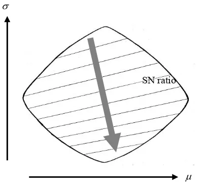
We can calculate the accumulated simultaneous distribution probability for each coefficient of variation (μ σ/ =0.01, 0.02, 0.05, 0.1, 0.2, 0.5, 0.75, 1.0) with the range of μ and σ from 0 to ∞. At the same time, SN ratio is calculated in accordance with the definition-equation of the nominal–the-best type character. With the reliability θ of the estimation, the region of F a
( )
≥0.5(1−θ) is illustrated in Figure 1.The boundary for the reliability of θ is shown in the circumference of the curved surface. Each internal line has the same SN ratio. It becomes the contour of SN ratio. The SN ratio increases towards the right and the bottom as shown by a big arrow in the figure. As the figure shows standard deviation in horizontal direction and mean in the vertical direction, the SN ratio increases with lower standard deviation and higher mean value. These contours are not quite parallel. They are skewed. Furthermore, the spacing is not equal. Let denote SN-R( )θ the SN ratio of the nominal-the-best type character inside this convex enclosed territory with the reliability of θ, then we define the difference of
SN-R( )θ by the following equation.
for the definition of the SN ratio. This shows that the
SN ratio changes according to the absolute factor level of its value. These influences can be mitigated by adopting above Δ( )θ . Moreover, for the SN ratio of nominal-the-best type character, average m and error dispersion Ve appear in the definition of SN-R( )θ , representing the mean μ and the standard deviation
σ , respectively, improving the transparency further.
Figure 1. Convex Enclosed Territory of the Accumulated Simultaneous Distribution (reliability θ)
and SN Ratio
Therefore, the space of reliability θ is obtained from the mean μ and standard deviation σ of the experiment data Yi. The hyper-plane of the SN ratio
within this space provides the maximum and minimum of the SN ratio.
4. Searching Method of Optimal Condition
4.1 Nominal-the-best Type Character
A nominal-the-best type character is evaluated by the small dispersion and closeness of the average to the desired value. We use the sensitivity index as an evaluation index of a nominal-the-best type character.
(Sensitivity) = 2
10 log(× m ) (6)
Note that the sensitivity index is not adopted for the lager-the-better and the smaller-the-better type characters.
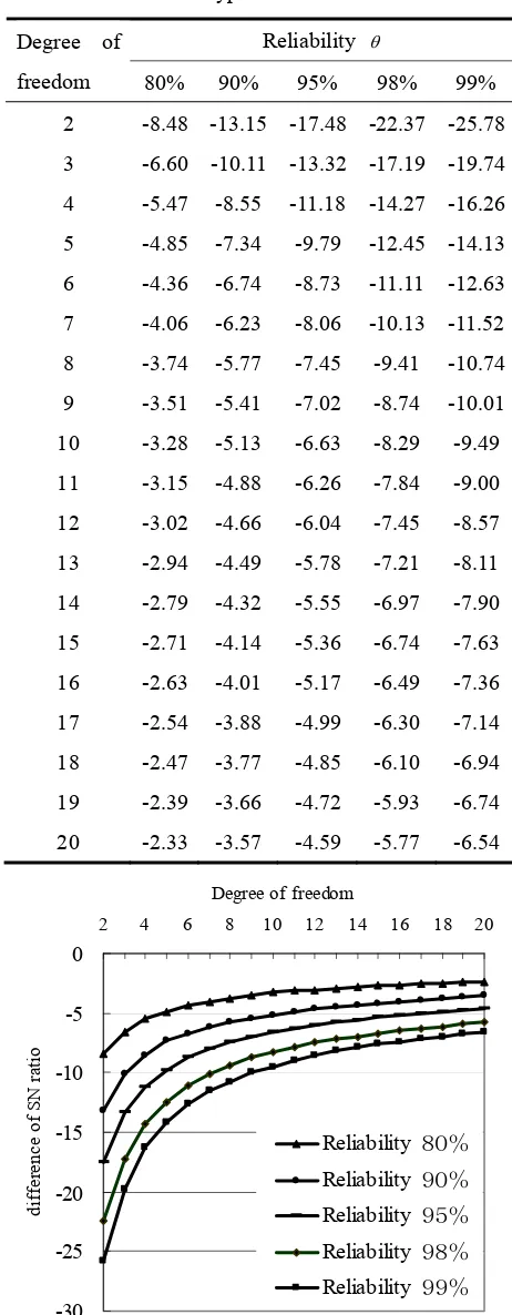
Above degree of freedom means the externally allocated orthogonal array, or a degree of freedom of the repetition. Note that SN-R( )θ changes with μ σ/ . But, it depends only on reliability θ without depending on
/
μ σ when it is evaluated with ( )Δθ . The calculated result is shown in Table 4 and Figure 2. The cases within the difference ( )Δθ from max SN-R( )θ are regarded as the candidate of the optimal case. When performing the confirmation test, it is strictly recommended to carry out these cases.
SN ratio
Table 4. The Difference of SN Ratio in the Nominal-the-best Type Characteristic Estimation
Reliability θ
Figure 2. Change of SN Ratio over the Reliability θ
4.2 Larger-the-better Type Character
As for the larger-the-better type character and the smaller-the-better type character as well, it can be treated in the same way. The failure avoidance procedure can apply in the same manner. You have only to be conscious with the difference of definition equation of SN ratio.
The nominal-the-best type character uses the mean and standard deviation independently in equation. This point is greatly different. The larger-the-better type character and the smaller-the-better type character do not contain these in the definition. Therefore, ( )Δθ changes by μ σ/ .
For the larger-the-better type character, it is considered to be good when the average is big and the dispersion is small. The following is the definition of the SN ratio of the larger-the- better type character.
2 2 2
As for this characteristic value as well, the dispersion of the SN ratio exists because of the sampling. Because the standard deviation is contained in the definition of the nominal-the-best type character,
( )θ
Δ by this sampling did not depend on coefficient of variation σ μ/ .
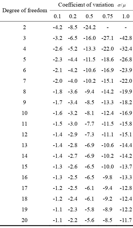
But, as for the larger-the-better type character discussed in this chapter, the value of ( )Δθ changes by coefficient of variation. The value of Δ( )θ in 90% reliability (risk level of 5% on each side) are obtained for the freedoms of 2 to 20, which is shown Figure 3 and Table 5.
Figure 3. Change of SN Ratio Over the Coefficient of Variance with 90% Reliability for Larger-the-better
-50
Table 5. The Difference of SN Ratio in the Larger-the- better Type with 90% Reliability
Coefficient of variation σ μ/ Degree of freedom
The influence of the change in the mean can be removed by using the difference between the maximum SN ratio and the minimum SN ratio. Figure 3 shows that as the degree of freedom increases, ( )Δθ becomes smaller. And ( )Δθ becomes smaller as the coefficient of variation σ μ/ gets smaller. ( )Δθ in other reliability θ can be obtained in the same way, too.
4.3 Smaller-the-better Type Character
As for the smaller-the-better type character, Δ( )θ by sampling is explained in the same way as the larger-the-better type character in the following. A smaller average and smaller dispersion are better in smaller-the-better type character. The following is the definition equation of the SN ratio of the smaller-the-better type character.
SN-ratio= − ×10 log(VT) (8)
where the characteristic value is positive, SN ratio becomes bigger as the average gets smaller. But, where
characteristic value is negative, the SN ratio becomes bigger as the average gets bigger. Within the positive territory, the SN ratio becomes bigger as the average and dispersion get smaller. The effect of correction termCT , the effect of a factor, and the error are included in the above definition of VT . The result
varies according to the balancing among those three effects. Furthermore, the dispersion of the SN ratio by the sampling also exists similar to what explained in the nominal-the-best type character. Because the standard deviation is contained in the definition of the nominal-the-best type character, ( )Δθ by this sampling did not depend on coefficient of variation
/
σ μ. As for the smaller-the- better type character being discussed in this chapter, the value of ( )Δθ changes by coefficient of variation.
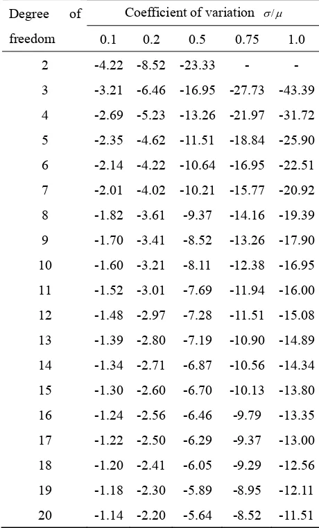
Figure 4 and Table 6 depict the change of the Δ( )θ with 90% reliability (risk level of 5% on each side) obtained for the freedoms of 2 to 20 for the smaller-the- better type characteristics. The influence of the variation of average is removed by using the difference between the maximum and minimum SN ratios, too. When a degree of freedom gets bigger, Δ( )θ becomes smaller in Figure 4. And, ( )Δθ becomes smaller, as the coefficient of variation σ μ/ gets smaller. ( )Δθ in other reliability can be obtained in the same manner, too.
Figure 4. Change of SN Ratio Over the Coefficient of Variance with 90% Reliability for Smaller-the-better
Type
5. Conclusion
procedure was proposed to solve this problem. The SN ratio is taken up as a comprehensive character which evaluates both average and dispersion at the same time. As shown in this report, there exists the danger that the order of preferred solution is derived in the wrong way when the average and dispersion are evaluated simultaneously. In the conventional statistics method, the average and dispersion are examined independently, but it is not the case when they are turned into SN ratio prior to the evaluation.
Table 6. The Difference of SN Ratio in the smaller-the-better Type with 90% Reliability
Coefficient of variation σ μ/ Degree of
freedom 0.1 0.2 0.5 0.75 1.0
2 -4.22 -8.52 -23.33 - -
3 -3.21 -6.46 -16.95 -27.73 -43.39
4 -2.69 -5.23 -13.26 -21.97 -31.72
5 -2.35 -4.62 -11.51 -18.84 -25.90
6 -2.14 -4.22 -10.64 -16.95 -22.51
7 -2.01 -4.02 -10.21 -15.77 -20.92
8 -1.82 -3.61 -9.37 -14.16 -19.39
9 -1.70 -3.41 -8.52 -13.26 -17.90
10 -1.60 -3.21 -8.11 -12.38 -16.95
11 -1.52 -3.01 -7.69 -11.94 -16.00
12 -1.48 -2.97 -7.28 -11.51 -15.08
13 -1.39 -2.80 -7.19 -10.90 -14.89
14 -1.34 -2.71 -6.87 -10.56 -14.34
15 -1.30 -2.60 -6.70 -10.13 -13.80
16 -1.24 -2.56 -6.46 -9.79 -13.35
17 -1.22 -2.50 -6.29 -9.37 -13.00
18 -1.20 -2.41 -6.05 -9.29 -12.56
19 -1.18 -2.30 -5.89 -8.95 -12.11
20 -1.14 -2.20 -5.64 -8.52 -11.51
Therefore, there is a possibility of adopting non- optimal condition as the optimum as the result of experiment. Another problem is that engineers in charge of testing can overlook it without noticing this danger. Because it was obtained as a fact, the result of the experiment tends to be treated as trustworthy in practice.
Research and development can be miss-lead by improper interpretation of experiment results. Those cases are often encountered in reality and treated as the
failed experiment. It is quite important to clarify precautions and prepare an improved method as the one in this paper.
Many people can be missing the optimal solution without notice and taking the ones of less importance. As the result, development fails leaving the self recognition of insufficient competence. The new method proposed here has a big advantage of preventing such losing of the best solution.
References
Miyagawa, M. (2006). Advanced course of the design of experiment. Tokyo: Nikkagiren Press.