When conducting monetary and fiscal policy, policymakers often look be-yond their own country’s borders. Even if domestic prosperity is their sole ob-jective, it is necessary for them to consider the rest of the world. The international flow of goods and services and the international flow of capital can affect an economy in profound ways. Policymakers ignore these effects at their peril.
In this chapter we extend our analysis of aggregate demand to include inter-national trade and finance. The model developed in this chapter, called the Mundell–Fleming model, is an open-economy version of the IS–LMmodel. Both models stress the interaction between the goods market and the money market. Both models assume that the price level is fixed and then show what causes short-run fluctuations in aggregate income (or, equivalently, shifts in the aggregate demand curve).The key difference is that the IS–LMmodel assumes a closed economy, whereas the Mundell–Fleming model assumes an open econ-omy.The Mundell–Fleming model extends the short-run model of national in-come from Chapters 10 and 11 by including the effects of international trade and finance from Chapter 5.
The Mundell–Fleming model makes one important and extreme assump-tion: it assumes that the economy being studied is a small open economy with perfect capital mobility.That is, the economy can borrow or lend as much as it wants in world financial markets and, as a result, the economy’s interest rate is determined by the world interest rate. One virtue of this assumption is that it simplifies the analysis: once the interest rate is determined, we can concentrate our attention on the role of the exchange rate. In addition, for some economies, such as Belgium or the Netherlands, the assumption of a small open economy with perfect capital mobility is a good one. Yet this assump-tion—and thus the Mundell–Fleming model—does not apply exactly to a large open economy such as the United States. In the conclusion to this chap-ter (and more fully in the appendix), we consider what happens in the more complex case in which international capital mobility is less than perfect or a nation is so large it can influence world financial markets.
One lesson from the Mundell–Fleming model is that the behavior of an econ-omy depends on the exchange-rate system it has adopted.We begin by assuming that the economy operates with a floating exchange rate.That is, we assume that the central bank allows the exchange rate to adjust to changing economic condi-tions.We then examine how the economy operates under a fixed exchange rate,
12
and we discuss whether a floating or fixed exchange rate is better.This question has been important in recent years, as many nations around the world have de-bated what exchange-rate system to adopt.
12-1
The Mundell–Fleming Model
In this section we build the Mundell–Fleming model, and in the following sec-tions we use the model to examine the impact of various policies. As you will see, the Mundell–Fleming model is built from components we have used in pre-vious chapters. But these pieces are put together in a new way to address a new set of questions.1
The Key Assumption: Small Open Economy With
Perfect Capital Mobility
Let’s begin with the assumption of a small open economy with perfect capital mobility. As we saw in Chapter 5, this assumption means that the interest rate in this economy r is determined by the world interest rate r*. Mathematically, we can write this assumption as
r =r*.
This world interest rate is assumed to be exogenously fixed because the economy is sufficiently small relative to the world economy that it can borrow or lend as much as it wants in world financial markets without affecting the world interest rate.
Although the idea of perfect capital mobility is expressed with a simple tion, it is important not to lose sight of the sophisticated process that this equa-tion represents. Imagine that some event were to occur that would normally raise the interest rate (such as a decline in domestic saving). In a small open economy, the domestic interest rate might rise by a little bit for a short time, but as soon as it did, foreigners would see the higher interest rate and start lending to this coun-try (by, for instance, buying this councoun-try’s bonds).The capital inflow would drive the domestic interest rate back toward r*. Similarly, if any event were ever to start driving the domestic interest rate downward, capital would flow out of the country to earn a higher return abroad, and this capital outflow would drive the domestic interest rate back upward toward r*. Hence, the r =r*equation repre-sents the assumption that the international flow of capital is rapid enough to keep the domestic interest rate equal to the world interest rate.
The Mundell–Fleming model describes the market for goods and services much as the IS–LMmodel does, but it adds a new term for net exports. In particular, the goods market is represented with the following equation:
Y=C(Y−T) +I(r*) +G+NX(e).
This equation states that aggregate income Yis the sum of consumption C, in-vestment I, government purchases G, and net exports NX. Consumption de-pends positively on disposable income Y−T. Investment depends negatively on the interest rate, which equals the world interest rate r*. Net exports depend negatively on the exchange rate e.As before, we define the exchange rate eas the amount of foreign currency per unit of domestic currency—for example, e might be 100 yen per dollar.
You may recall that in Chapter 5 we related net exports to the real exchange rate (the relative price of goods at home and abroad) rather than the nominal ex-change rate (the relative price of domestic and foreign currencies). If e is the nominal exchange rate, then the real exchange rate
e
equals eP/P*, where P is the domestic price level and P*is the foreign price level.The Mundell–Fleming model, however, assumes that the price levels at home and abroad are fixed, so the real exchange rate is proportional to the nominal exchange rate. That is, when the nominal exchange rate appreciates (say, from 100 to 120 yen per dol-lar), foreign goods become cheaper compared to domestic goods, and this causes exports to fall and imports to rise.We can illustrate this equation for goods market equilibrium on a graph in which income is on the horizontal axis and the exchange rate is on the vertical axis.This curve is shown in panel (c) of Figure 12-1 and is called the IS*curve. The new label reminds us that the curve is drawn holding the interest rate con-stant at the world interest rate r*.
The IS*curve slopes downward because a higher exchange rate reduces net exports, which in turn lowers aggregate income. To show how this works, the other panels of Figure 12-1 combine the net-exports schedule and the Keynes-ian cross to derive the IS* curve. In panel (a), an increase in the exchange rate from e1to e2lowers net exports from NX(e1) to NX(e2). In panel (b), the reduc-tion in net exports shifts the planned-expenditure schedule downward and thus lowers income from Y1 to Y2. The IS* curves summarizes this relationship be-tween the exchange rate eand income Y.
The Money Market and the
LM*
Curve
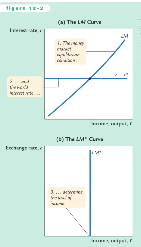
The Mundell–Fleming model represents the money market with an equation that should be familiar from the IS–LMmodel, with the additional assumption that the domestic interest rate equals the world interest rate:
This equation states that the supply of real money balances,M/P, equals the demand,L(r,Y). The demand for real balances depends negatively on the in-terest rate, which is now set equal to the world inin-terest rate r*, and positively on income Y. The money supply M is an exogenous variable controlled by the central bank, and because the Mundell–Fleming model is designed to an-alyze short-run fluctuations, the price level P is also assumed to be exoge-nously fixed.
We can represent this equation graphically with a vertical LM* curve, as in panel (b) of Figure 12-2. The LM* curve is vertical because the exchange rate does not enter into the LM* equation. Given the world interest rate, the LM* equation determines aggregate income, regardless of the exchange rate. Figure 12-2 shows how the LM* curve arises from the world interest rate and the LM curve, which relates the interest rate and income.
f i g u r e 1 2 - 1 changes in the goods market equilibrium. schedule and the Keynesian cross. Panel (a) shows the net-exports schedule: an increase in the exchange rate from e1to e2lowers net exports from NX(e1) to NX(e2). Panel (b) shows the Keynesian cross: a decrease in net exports from
Putting the Pieces Together
According to the Mundell–Fleming model, a small open economy with perfect capital mobility can be described by two equations:
Y=C(Y−T) +I(r*) +G+NX(e) IS*, M/P=L(r*,Y) LM*.
The first equation describes equilibrium in the goods market, and the second equation describes equilibrium in the money market. The exogenous variables are fiscal policy Gand T, monetary policy M, the price level P, and the world
in-terest rate r*.The endogenous variables are income Yand the exchange rate e.
Figure 12-3 illustrates these two relationships.The equilibrium for the
econ-Interest rate, r
Exchange rate, e
Income, output, Y
Income, output, Y
1. The money market equilibrium condition . . .
2. . . . and the world interest rate . . .
3. . . . determine the level of income.
(a) The LM Curve
(b) The LM* Curve
LM
r ⫽ r*
LM*
shows the exchange rate and the level of income at which both the goods market and the money market are in equilibrium. With this diagram, we can use the Mundell–Fleming model to show how aggregate income Y and the exchange rate erespond to changes in policy.
12-2
The Small Open Economy Under Floating
Exchange Rates
Before analyzing the impact of policies in an open economy, we must specify the international monetary system in which the country has chosen to operate. We start with the system relevant for most major economies today: floating ex-change rates. Under floating exchange rates, the exchange rate is allowed to fluctuate in response to changing economic conditions.
Fiscal Policy
Suppose that the government stimulates domestic spending by increasing govern-ment purchases or by cutting taxes. Because such expansionary fiscal policy in-creases planned expenditure, it shifts the IS*curve to the right, as in Figure 12-4. As a result, the exchange rate appreciates, whereas the level of income remains the same.
Notice that fiscal policy has very different effects in a small open economy than it does in a closed economy. In the closed-economy IS–LM model, a fiscal expansion raises income, whereas in a small open economy with a floating exchange rate, a fiscal expansion leaves income at the same level. Why the
f i g u r e 1 2 - 3
Exchange rate, e
Income, output,Y Equilibrium
exchange rate
Equilibrium income
LM*
IS*
The Mundell–Fleming Model
difference? When income rises in a closed economy, the interest rate rises, because higher income increases the demand for money.That is not possible in a small open economy: as soon as the interest rate tries to rise above the world interest rate r*, capital flows in from abroad.This capital inflow increases the
de-mand for the domestic currency in the market for foreign-currency exchange and, thus, bids up the value of the domestic currency.The appreciation of the ex-change rate makes domestic goods expensive relative to foreign goods, and this reduces net exports.The fall in net exports offsets the effects of the expansionary
fiscal policy on income.
Why is the fall in net exports so great that it renders fiscal policy powerless to influence income? To answer this question, consider the equation that describes the money market:
M/P=L(r,Y).
In both closed and open economies, the quantity of real money balances sup-plied M/P is fixed, and the quantity demanded (determined by rand Y) must
equal this fixed supply. In a closed economy, a fiscal expansion causes the equilibrium interest rate to rise. This increase in the interest rate (which re-duces the quantity of money demanded) allows equilibrium income to rise (which increases the quantity of money demanded). By contrast, in a small open economy, r is fixed at r*, so there is only one level of income that
can satisfy this equation, and this level of income does not change when fiscal policy changes. Thus, when the government increases spending or cuts taxes, the appreciation of the exchange rate and the fall in net exports must be large enough to offset fully the normal expansionary effect of the policy on income.
Exchange rate, e
Income, output,Y Equilibrium
exchange rate
LM*
IS*2
IS*1 2. . . . which
raises the exchange
rate . . . 3. . . . and leaves income unchanged.
1. Expansionary fiscal policy shifts the IS* curve to the right, . . .
A Fiscal Expansion Under Floating Exchange Rates An increase in government
Monetary Policy
Suppose now that the central bank increases the money supply. Because the price level is assumed to be fixed, the increase in the money supply means an increase in real balances.The increase in real balances shifts the LM*curve to the right, as in Figure 12-5. Hence, an increase in the money supply raises income and lowers the exchange rate.
f i g u r e 1 2 - 5
Exchange rate, e
Income, output, Y
2. . . . which lowers the exchange rate . . .
3. . . . and raises income.
1. A monetary expan-sion shifts the LM* curve to the right, . . . LM*1
IS* LM*2
A Monetary Expansion Under Floating Exchange Rates An increase in the money supply shifts the LM*curve to the right, lowering the exchange rate and raising income.
Although monetary policy influences income in an open economy, as it does in a closed economy, the monetary transmission mechanism is different. Recall that in a closed economy an increase in the money supply increases spending be-cause it lowers the interest rate and stimulates investment. In a small open econ-omy, the interest rate is fixed by the world interest rate. As soon as an increase in the money supply puts downward pressure on the domestic interest rate, capital flows out of the economy as investors seek a higher return elsewhere.This capital outflow prevents the domestic interest rate from falling. In addition, because the capital outflow increases the supply of the domestic currency in the market for foreign-currency exchange, the exchange rate depreciates. The fall in the ex-change rate makes domestic goods inexpensive relative to foreign goods and, thereby, stimulates net exports. Hence, in a small open economy, monetary policy influences income by altering the exchange rate rather than the interest rate.
Trade Policy
Suppose that the government reduces the demand for imported goods by impos-ing an import quota or a tariff. What happens to aggregate income and the ex-change rate?
right, as in Figure 12-6. This shift in the net-exports schedule increases planned expenditure and thus moves the IS* curve to the right. Because the LM* curve is vertical, the trade restriction raises the exchange rate but does
not affect income.
Often a stated goal of policies to restrict trade is to alter the trade balance NX.
Yet, as we first saw in Chapter 5, such policies do not necessarily have that effect. The same conclusion holds in the Mundell–Fleming model under floating ex-change rates. Recall that
NX(e) =Y−C(Y−T) −I(r*) −G.
Exchange rate, e
Exchange rate, e
Net exports, NX
Income, output, Y NX2
NX1
IS*2 LM*
IS*1 3. . . . increasing
the exchange rate . . .
4. . . . and leaving income the same.
(a) The Shift in the Net-Exports Schedule
1. A trade restriction shifts the NX curve outward, . . .
(b) The Change in the Economy,s Equilibrium
2. . . . which shifts the IS* curve outward, . . .
Because a trade restriction does not affect income, consumption, investment, or government purchases, it does not affect the trade balance. Although the shift in the net-exports schedule tends to raise NX, the increase in the exchange rate
re-duces NXby the same amount.
12-3
The Small Open Economy Under Fixed
Exchange Rates
We now turn to the second type of exchange-rate system: fixed exchange
rates. In the 1950s and 1960s, most of the world’s major economies, including the United States, operated within the Bretton Woods system—an international
monetary system under which most governments agreed to fix exchange rates.
The world abandoned this system in the early 1970s, and exchange rates were al-lowed to float. Some European countries later reinstated a system of fixed ex-change rates among themselves, and some economists have advocated a return to a worldwide system of fixed exchange rates. In this section we discuss how such a system works, and we examine the impact of economic policies on an econ-omy with a fixed exchange rate.
How a Fixed-Exchange-Rate System Works
Under a system of fixed exchange rates, a central bank stands ready to buy or sell the domestic currency for foreign currencies at a predetermined price. For ex-ample, suppose that the Fed announced that it was going to fix the exchange rate at 100 yen per dollar. It would then stand ready to give $1 in exchange for 100 yen or to give 100 yen in exchange for $1. To carry out this policy, the Fed would need a reserve of dollars (which it can print) and a reserve of yen (which it must have purchased previously).
A fixed exchange rate dedicates a country’s monetary policy to the single goal of keeping the exchange rate at the announced level. In other words, the essence of a fixed-exchange-rate system is the commitment of the central bank to allow the money supply to adjust to whatever level will ensure that the equilibrium exchange rate equals the announced exchange rate. More-over, as long as the central bank stands ready to buy or sell foreign currency at the fixed exchange rate, the money supply adjusts automatically to the neces-sary level.
rise in the money supply shifts the LM*curve to the right, lowering the equilib-rium exchange rate. In this way, the money supply continues to rise until the equilibrium exchange rate falls to the announced level.
Conversely, suppose that when the Fed announces that it will fix the ex-change rate at 100 yen per dollar, the equilibrium is 50 yen per dollar. Panel (b) of Figure 12-7 shows this situation. In this case, an arbitrageur could make a profit by buying 100 yen from the Fed for $1 and then selling the yen in the marketplace for $2. When the Fed sells these yen, the $1 it receives automati-cally reduces the money supply. The fall in the money supply shifts the LM*
curve to the left, raising the equilibrium exchange rate. The money supply continues to fall until the equilibrium exchange rate rises to the announced level.
It is important to understand that this exchange-rate system fixes the nominal exchange rate. Whether it also fixes the real exchange rate depends on the time horizon under consideration. If prices are flexible, as they are in the long run, then the real exchange rate can change even while the nominal exchange rate is fixed. Therefore, in the long run described in Chapter 5, a policy to fix the nominal exchange rate would not influence any real variable, including the real exchange rate. A fixed nominal exchange rate would influence only the money supply and the price level.Yet in the short run described by the Mundell–Fleming model, prices are fixed, so a fixed nominal exchange rate implies a fixed real exchange rate as well.
Exchange rate, e Exchange rate, e
Income, output, Y Income, output, Y
Equilibrium exchange rate
Fixed exchange rate
Fixed exchange rate
Equilibrium exchange rate
(a) The Equilibrium Exchange Rate Is Greater Than the Fixed Exchange Rate
LM*1 LM*2 LM*2 LM*1
IS*
(b) The Equilibrium Exchange Rate Is Less Than the Fixed Exchange Rate
IS*
Fiscal Policy
Let’s now examine how economic policies affect a small open economy with a
fixed exchange rate. Suppose that the government stimulates domestic spending by increasing government purchases or by cutting taxes.This policy shifts the IS*
curve to the right, as in Figure 12-8, putting upward pressure on the exchange rate. But because the central bank stands ready to trade foreign and domestic cur-rency at the fixed exchange rate, arbitrageurs quickly respond to the rising ex-change rate by selling foreign currency to the central bank, leading to an automatic monetary expansion. The rise in the money supply shifts the LM*
curve to the right.Thus, under a fixed exchange rate, a fiscal expansion raises ag-gregate income.
C A S E S T U D Y
The International Gold Standard
During the late nineteenth and early twentieth centuries, most of the world’s major economies operated under a gold standard. Each country maintained a re-serve of gold and agreed to exchange one unit of its currency for a specified amount of gold.Through the gold standard, the world’s economies maintained a system of fixed exchange rates.
To see how an international gold standard fixes exchange rates, suppose that the U.S. Treasury stands ready to buy or sell 1 ounce of gold for $100, and the Bank of England stands ready to buy or sell 1 ounce of gold for 100 pounds.To-gether, these policies fix the rate of exchange between dollars and pounds: $1 must trade for 1 pound. Otherwise, the law of one price would be violated, and it would be profitable to buy gold in one country and sell it in the other.
For example, suppose that the exchange rate were 2 pounds per dollar. In this case, an arbitrageur could buy 200 pounds for $100, use the pounds to buy 2 ounces of gold from the Bank of England, bring the gold to the United States, and sell it to the Treasury for $200—making a $100 profit. Moreover, by bringing the gold to the United States from England, the arbitrageur would in-crease the money supply in the United States and dein-crease the money supply in England.
Thus, during the era of the gold standard, the international transport of gold by arbitrageurs was an automatic mechanism adjusting the money supply and stabilizing exchange rates. This system did not completely fix exchange rates, because shipping gold across the Atlantic was costly.Yet the international gold standard did keep the exchange rate within a range dictated by trans-portation costs. It thereby prevented large and persistent movements in ex-change rates.2
2 For more on how the gold standard worked, see the essays in Barry Eichengreen, ed.,The Gold
2. . . . a fiscal fiscal expansion shifts the IS*
curve to the right. To maintain the fixed exchange rate, the Fed must increase the money supply, thereby shifting the LM*curve to the right. Hence, in contrast to the case of floating exchange rates, under fixed exchange rates a fiscal expansion raises income. Fixed Exchange Rates If the Fed tries to increase the money supply—for example, by buying bonds from the public—it will put downward pressure on the exchange rate. To maintain the fixed exchange rate, the money supply and the LM*curve must return to their initial positions. Hence, under fixed exchange rates, normal monetary policy is ineffectual.
Monetary Policy
rate, arbitrageurs quickly respond to the falling exchange rate by selling the
do-mestic currency to the central bank, causing the money supply and the LM*
curve to return to their initial positions. Hence, monetary policy as usually con-ducted is ineffectual under a fixed exchange rate. By agreeing to fix the exchange rate, the central bank gives up its control over the money supply.
A country with a fixed exchange rate can, however, conduct a type of
mone-tary policy: it can decide to change the level at which the exchange rate is fixed.
A reduction in the value of the currency is called a devaluation, and an increase
in its value is called a revaluation. In the Mundell–Fleming model, a
devalua-tion shifts the LM* curve to the right; it acts like an increase in the money
sup-ply under a floating exchange rate. A devaluation thus expands net exports and
raises aggregate income. Conversely, a revaluation shifts the LM* curve to the
left, reduces net exports, and lowers aggregate income.
C A S E S T U D Y
Devaluation and the Recovery From the Great Depression
The Great Depression of the 1930s was a global problem.Although events in the
United States may have precipitated the downturn, all of the world’s major
economies experienced huge declines in production and employment.Yet not all governments responded to this calamity in the same way.
One key difference among governments was how committed they were to
the fixed exchange rate set by the international gold standard. Some countries,
such as France, Germany, Italy, and the Netherlands, maintained the old rate of exchange between gold and currency. Other countries, such as Denmark, Fin-land, Norway, Sweden, and the United Kingdom, reduced the amount of gold they would pay for each unit of currency by about 50 percent. By reducing the gold content of their currencies, these governments devalued their currencies relative to those of other countries.
The subsequent experience of these two groups of countries conforms to the
prediction of the Mundell–Fleming model.Those countries that pursued a
pol-icy of devaluation recovered quickly from the Depression.The lower value of the currency raised the money supply, stimulated exports, and expanded production. By contrast, those countries that maintained the old exchange rate suffered
longer with a depressed level of economic activity.3
3
Barry Eichengreen and Jeffrey Sachs,“Exchange Rates and Economic Recovery in the 1930s,” Journal of Economic History45 (December 1985): 925–946.
Trade Policy
Suppose that the government reduces imports by imposing an import quota or a tariff. This policy shifts the net-exports schedule to the right and thus shifts the
raise the exchange rate.To keep the exchange rate at the fixed level, the money supply must rise, shifting the LM*curve to the right.
The result of a trade restriction under a fixed exchange rate is very different from that under a floating exchange rate. In both cases, a trade restriction shifts the net-exports schedule to the right, but only under a fixed exchange rate does a trade restriction increase net exports NX.The reason is that a trade restriction under a fixed exchange rate induces monetary expansion rather than an appreci-ation of the exchange rate.The monetary expansion, in turn, raises aggregate in-come. Recall the accounting identity
NX=S−I.
When income rises, saving also rises, and this implies an increase in net exports.
Policy in the Mundell–Fleming Model: A Summary
The Mundell–Fleming model shows that the effect of almost any economic pol-icy on a small open economy depends on whether the exchange rate is floating or fixed. Table 12-1 summarizes our analysis of the short-run effects of fiscal, monetary, and trade policies on income, the exchange rate, and the trade balance. What is most striking is that all of the results are different under floating and
fixed exchange rates.
To be more specific, the Mundell–Fleming model shows that the power of monetary and fiscal policy to influence aggregate income depends on the exchange-rate regime. Under floating exchange rates, only monetary policy can affect income.The usual expansionary impact of fiscal policy is offset by a rise in Exchange rate,e
Income, output,Y 1. With
a fixed exchange rate, . . .
2. . . . a trade restriction shifts the IS* curve to the right, . . .
3. . . . which induces a shift in the LM* curve . . .
IS*1 IS*2 LM*2
LM*1
Y2 Y1
4. . . . and raises income.
the value of the currency. Under fixed exchange rates, only fiscal policy can af-fect income.The normal potency of monetary policy is lost because the money supply is dedicated to maintaining the exchange rate at the announced level.
12-4
Interest-Rate Differentials
So far, our analysis has assumed that the interest rate in a small open economy is equal to the world interest rate:r=r*.To some extent, however, interest rates dif-fer around the world.We now extend our analysis by considering the causes and effects of international interest-rate differentials.
Country Risk and Exchange-Rate Expectations
When we assumed earlier that the interest rate in our small open economy is de-termined by the world interest rate, we were applying the law of one price.We rea-soned that if the domestic interest rate were above the world interest rate, people from abroad would lend to that country, driving the domestic interest rate down. And if the domestic interest rate were below the world interest rate, domestic resi-dents would lend abroad to earn a higher return, driving the domestic interest rate up. In the end, the domestic interest rate would equal the world interest rate.
Why doesn’t this logic always apply? There are two reasons.
One reason is country risk. When investors buy U.S. government bonds or make loans to U.S. corporations, they are fairly confident that they will be repaid with interest. By contrast, in some less developed countries, it is plausible to fear that a revolution or other political upheaval might lead to a default on loan re-payments. Borrowers in such countries often have to pay higher interest rates to compensate lenders for this risk.
EXCHANGE-RATE REGIME FLOATING FIXED
IMPACT ON:
Policy Y e NX Y e NX
Fiscal expansion 0 ↑ ↓ ↑ 0 0
Monetary expansion ↑ ↓ ↑ 0 0 0
Import restriction 0 ↑ 0 ↑ 0 ↑
Note: This table shows the direction of impact of various economic policies on income Y, the
exchange rate e, and the trade balance NX. A “↑” indicates that the variable increases; a “↓”
indicates that it decreases; a “0’’ indicates no effect. Remember that the exchange rate is defined as the amount of foreign currency per unit of domestic currency (for example, 100 yen per dollar).
exchange rate. For example, suppose that people expect the French franc to fall in value relative to the U.S. dollar.Then loans made in francs will be repaid in a less valuable currency than loans made in dollars. To compensate for this ex-pected fall in the French currency, the interest rate in France will be higher than the interest rate in the United States.
Thus, because of both country risk and expectations of future exchange-rate changes, the interest rate of a small open economy can differ from interest rates in other economies around the world. Let’s now see how this fact affects our analysis.
Differentials in the Mundell
–
Fleming Model
To incorporate interest-rate differentials into the Mundell–Fleming model, we assume that the interest rate in our small open economy is determined by the world interest rate plus a risk premium
v
:r=r*+
v
.The risk premium is determined by the perceived political risk of making loans in a country and the expected change in the real exchange rate. For our purposes here, we can take the risk premium as exogenous in order to examine how changes in the risk premium affect the economy.
The model is largely the same as before.The two equations are
Y=C(Y−T) +I(r*+
v
) +G+NX(e) IS*, M/P=L(r*+v
,Y) LM*.For any given fiscal policy, monetary policy, price level, and risk premium, these two equations determine the level of income and exchange rate that equilibrate the goods market and the money market. Holding constant the risk premium, the tools of monetary, fiscal, and trade policy work as we have already seen.
Now suppose that political turmoil causes the country’s risk premium
v
to rise.The most direct effect is that the domestic interest rate rrises.The higherin-terest rate, in turn, has two effects. First, the IS*curve shifts to the left, because
the higher interest rate reduces investment. Second, the LM* curve shifts to the
right, because the higher interest rate reduces the demand for money, and this al-lows a higher level of income for any given money supply. [Recall that Y must
satisfy the equation M/P=L(r*+
v
,Y).] As Figure 12-11 shows, these two shiftscause income to rise and the currency to depreciate.
up French interest rates and, as we have just seen, will drive down the value of the French currency.Thus, the expectation that a currency will lose value in the future causes it to lose value today.
One surprising—and perhaps inaccurate—prediction of this analysis is that an increase in country risk as measured by
v
will cause the economy’s income to in-crease. This occurs in Figure 12-11 because of the rightward shift in the LM* curve. Although higher interest rates depress investment, the depreciation of the currency stimulates net exports by an even greater amount. As a result, aggregate income rises.There are three reasons why, in practice, such a boom in income does not occur. First, the central bank might want to avoid the large depreciation of the domestic currency and, therefore, may respond by decreasing the money sup-ply M. Second, the depreciation of the domestic currency may suddenly in-crease the price of imported goods, causing an inin-crease in the price level P. Third, when some event increases the country risk premium
v
, residents of the country might respond to the same event by increasing their demand for money (for any given income and interest rate), because money is often the safest asset available. All three of these changes would tend to shift the LM* curve toward the left, which mitigates the fall in the exchange rate but also tends to depress income.Thus, increases in country risk are not desirable. In the short run, they typi-cally lead to a depreciating currency and, through the three channels just de-scribed, falling aggregate income. In addition, because a higher interest rate reduces investment, the long-run implication is reduced capital accumulation and lower economic growth.
International Financial Crisis: Mexico 1994–1995
In August 1994, a Mexican peso was worth 30 cents. A year later, it was worth only 16 cents. What explains this massive fall in the value of the Mexican cur-rency? Country risk is a large part of the story.
At the beginning of 1994, Mexico was a country on the rise.The recent pas-sage of the North American Free Trade Agreement (NAFTA), which reduced trade barriers among the United States, Canada, and Mexico, made many confi -dent about the future of the Mexican economy. Investors around the world were eager to make loans to the Mexican government and to Mexican corporations.
Political developments soon changed that perception. A violent uprising in the Chiapas region of Mexico made the political situation in Mexico seem pre-carious.Then Luis Donaldo Colosio, the leading presidential candidate, was assas-sinated. The political future looked less certain, and many investors started placing a larger risk premium on Mexican assets.
At first, the rising risk premium did not affect the value of the peso, because Mexico was operating with a fixed exchange rate.As we have seen, under a fixed exchange rate, the central bank agrees to trade the domestic currency (pesos) for a foreign currency (dollars) at a predetermined rate. Thus, when an increase in the country risk premium put downward pressure on the value of the peso, the Mexican central bank had to accept pesos and pay out dollars. This automatic exchange-market intervention contracted the Mexican money supply (shifting the LM*curve to the left) when the currency might otherwise have depreciated. Yet Mexico’s reserves of foreign currency were too small to maintain its fixed exchange rate. When Mexico ran out of dollars at the end of 1994, the Mexican government announced a devaluation of the peso. This decision had repercus-sions, however, because the government had repeatedly promised that it would not devalue. Investors became even more distrustful of Mexican policymakers and feared further Mexican devaluations.
Investors around the world (including those in Mexico) avoided buying Mex-ican assets. The country risk premium rose once again, adding to the upward pressure on interest rates and the downward pressure on the peso.The Mexican stock market plummeted. When the Mexican government needed to roll over some of its debt that was coming due, investors were unwilling to buy the new debt. Default appeared to be the government’s only option. In just a few months, Mexico had gone from being a promising emerging economy to being a risky economy with a government on the verge of bankruptcy.
due.These loan guarantees helped restore confidence in the Mexican economy, thereby reducing to some extent the country risk premium.
Although the U.S. loan guarantees may well have stopped a bad situation from getting worse, they did not prevent the Mexican meltdown of 1994–1995 from being a painful experience for the Mexican people. Not only did the Mexican currency lose much of its value, but Mexico also went through a deep recession. Fortunately, by the late 1990s, aggregate income was growing again, and the worst appeared to be over. But the lesson from this experience is clear and could well apply again in the future: changes in perceived country risk, often attribut-able to political instability, are an important determinant of interest rates and ex-change rates in small open economies.
C A S E S T U D Y
International Financial Crisis: Asia 1997–1998
In 1997, as the Mexican economy was recovering from its financial crisis, a similar story started to unfold in several Asian economies, including Thailand, South Korea, and especially Indonesia. The symptoms were familiar: high interest rates, falling asset values, and a depreciating currency. In Indonesia, for instance, short-term nom-inal interest rates rose above 50 percent, the stock market lost about 90 percent of its value (measured in U.S. dollars), and the rupiah fell against the dollar by more than 80 percent.The crisis led to rising inflation in these countries (because the depreci-ating currency made imports more expensive) and to falling GDP (because high in-terest rates and reduced confidence depressed spending). Real GDP in Indonesia fell about 13 percent in 1998, making the downturn larger than any U.S. recession since the Great Depression of the 1930s.
What sparked this firestorm? The problem began in the Asian banking systems. For many years, the governments in the Asian nations had been more involved in managing the allocation of resources—in particular,financial resources—than is true in the United States and other developed countries. Some commentators had applauded this “partnership”between government and private enterprise and had even suggested that the United States should follow the example. Over time, however, it became clear that many Asian banks had been extending loans to those with the most political clout rather than to those with the most profitable invest-ment projects. Once rising default rates started to expose this “crony capitalism,”
as it was then called, international investors started to lose confidence in the future of these economies.The risk premiums for Asian assets rose, causing interest rates to skyrocket and currencies to collapse.
International crises of confidence often involve a vicious circle that can am-plify the problem. Here is one story about what happened in Asia:
1.Problems in the banking system eroded international confidence in these economies.
12-5
Should Exchange Rates Be Floating
or Fixed?
Having analyzed how an economy works under floating and fixed exchange rates, let’s consider which exchange-rate regime is better.
Pros and Cons of Different Exchange-Rate Systems
The primary argument for a floating exchange rate is that it allows monetary pol-icy to be used for other purposes. Under fixed rates, monetary policy is commit-ted to the single goal of maintaining the exchange rate at its announced level.Yet the exchange rate is only one of many macroeconomic variables that monetary policy can influence. A system of floating exchange rates leaves monetary policy-makers free to pursue other goals, such as stabilizing employment or prices.
Advocates of fixed exchange rates argue that exchange-rate uncertainty makes international trade more difficult. After the world abandoned the Bretton Woods system of fixed exchange rates in the early 1970s, both real and nominal exchange rates became (and remained) much more volatile than anyone had expected. Some economists attribute this volatility to irrational and destabilizing specula-tion by internaspecula-tional investors. Business executives often claim that this volatility is harmful because it increases the uncertainty that accompanies international business transactions. Yet, despite this exchange-rate volatility, the amount of world trade has continued to rise under floating exchange rates.
of stock and other assets.
4.Falling asset prices reduced the value of collateral being used for bank loans.
5.Reduced collateral increased default rates on bank loans.
6.Greater defaults exacerbated problems in the banking system. Now return to
step 1 to complete and continue the circle.
Some economists have used this vicious-circle argument to suggest that the Asian crisis was a self-fulfilling prophecy: bad things happened merely because people expected bad things to happen. Most economists, however, thought the political corruption of the banking system was a real problem, which was then compounded by this vicious circle of reduced confidence.
Advocates of fixed exchange rates sometimes
argue that a commitment to a fixed exchange rate
is one way to discipline a nation’s monetary
au-thority and prevent excessive growth in the money supply. Yet there are many other policy rules to which the central bank could be com-mitted. In Chapter 14, for instance, we discuss policy rules such as targets for nominal GDP or
the inflation rate. Fixing the exchange rate has the
advantage of being simpler to implement than these other policy rules, because the money sup-ply adjusts automatically, but this policy may lead to greater volatility in income and employment.
In the end, the choice between floating and
fixed rates is not as stark as it may seem at first.
During periods of fixed exchange rates, countries
can change the value of their currency if
main-taining the exchange rate conflicts too severely
with other goals. During periods of floating
ex-change rates, countries often use formal or
infor-mal targets for the exchange rate when deciding whether to expand or contract
the money supply.We rarely observe exchange rates that are completely fixed or
completely floating. Instead, under both systems, stability of the exchange rate is
usually one among many of the central bank’s objectives.
“Then it’s agreed. Until the dollar firms up, we let the clamshell float.”
© The New Y
or
ker collection 1971 Ed Fisher fr
om car
toonbank
.com. All Rights Reser
ved.
C A S E S T U D Y
Monetary Union in the United States and Europe
If you have ever driven the 3,000 miles from New York City to San Francisco, you may recall that you never needed to change your money from one form of currency
to another. In all fifty U.S. states, local residents are happy to accept the U.S. dollar
for the items you buy. Such a monetary unionis the most extreme form of a fixed
ex-change rate.The exex-change rate between New York dollars and San Francisco dollars
is so irrevocably fixed that you may not even know that there is a difference
be-tween the two. (What’s the difference? Each dollar bill is issued by one of the dozen
local Federal Reserve Banks.Although the bank of origin can be identified from the
bill’s markings, you don’t care which type of dollar you hold because everyone else,
including the Federal Reserve system, is ready to trade them one for one.)
If you have ever made a similar 3,000-mile trip across Europe, however, your
ex-perience was probably very different.You didn’t have to travel far before needing to
Speculative Attacks, Currency Boards, and Dollarization
Imagine that you are a central banker of a small country. You and your fellow policymakers decide to fix your currency—let’s call it the peso—against the U.S. dollar. From now on, one peso will sell for one dollar.
As we discussed earlier, you now have to stand ready to buy and sell pesos for a dollar each. The money supply will adjust automatically to make the equilib-rium exchange rate equal your target. There is, however, one potential problem with this plan: you might run out of dollars. If people come to the central bank extension of the European Monetary System (EMS), which during the previous two decades had attempted to limit exchange-rate fluctuations among participat-ing countries.When the euro is fully adopted, this goal will be achieved: the ex-change rate between France and Germany will be as fixed as the exchange rate between New York City and San Francisco.
The introduction of a common currency has its costs.The most important is that the nations of Europe will no longer be able to conduct their own monetary policies. Instead, a European central bank, with participation of all member countries, will set a single monetary policy for all of Europe.The central banks of the individual countries will play a role similar to that of regional Federal Re-serve Banks: they will monitor local conditions but they will have no control over the money supply or interest rates. Critics of the move toward a common currency argue that the cost of losing national monetary policy is large. If a re-cession hits one country but not others in Europe, that country may wish it had the tool of monetary policy to combat the downturn.
Why, according to these economists, is monetary union a bad idea for Europe if it works so well in the United States? These economists argue that the United States is different from Europe in two important ways. First, labor is more mobile among U.S. states than among European countries.This is in part because the United States has a common language and in part because most Americans are descended from immigrants, who have shown a willingness to move.Therefore, when a regional re-cession occurs, U.S. workers are more likely to move from high-unemployment states to low-unemployment states. Second, the United States has a strong central government that can use fiscal policy—such as the federal income tax—to redistrib-ute resources among regions. Because Europe does not have these two advantages, it will suffer more when it restricts itself to a single monetary policy.
to sell large quantities of pesos, the central bank’s dollar reserves might dwindle to zero. In this case, the central bank has no choice but to abandon the fixed ex-change rate and let the peso depreciate.
This fact raises the possibility of a speculative attack—a change in investors’ per-ceptions that makes the fixed exchange rate untenable. Suppose that, for no good reason, a rumor spreads that the central bank is going to abandon the exchange-rate peg. People would respond by rushing to the central bank to convert pesos into dollars before the pesos lose value.This rush would drain the central bank’s reserves and could force the central bank to abandon the peg. In this case, the rumor would prove self-fulfilling.
To avoid this possibility, some economists argue that a fixed exchange rate should be supported by a currency board, such as that used by Argentina in the 1990s. A currency board is an arrangement by which the central bank holds enough for-eign currency to back each unit of the domestic currency. In our example, the cen-tral bank would hold one U.S. dollar (or one dollar invested in a U.S. government bond) for every peso. No matter how many pesos turned up at the central bank to be exchanged, the central bank would never run out of dollars.
Once a central bank has adopted a currency board, it might consider the natural next step: it can abandon the peso altogether and let its country use the U.S. dollar. Such a plan is called dollarization. It happens on its own in high-inflation economies, where foreign currencies offer a more reliable store of value than the domestic currency. But it can also occur as a matter of public policy: Panama is an example. If a country really wants its currency to be irrevocably fixed to the dollar, the most reliable method is to make its currency the dollar.The only loss from dollarization is the small seigniorage revenue, which accrues to the U.S. government.4
12-6
The Mundell
–
Fleming Model With a
Changing Price Level
So far we have been using the Mundell–Fleming model to study the small open economy in the short run when the price level is fixed. To see how this model relates to models we have examined previously, let’s consider what happens when the price level changes.
To examine price adjustment in an open economy, we must distinguish be-tween the nominal exchange rate e and the real exchange rate
e
, which equals eP/P*.We can write the Mundell–Fleming model asY=C(Y−T) +I(r*) +G+NX(
e
) IS*,M/P=L(r*,Y) LM*.
4 Dollarization may also lead to a loss in national pride from seeing American portraits on the
curve, and the second equation describes the *curve. Note that net exports depend on the real exchange rate.
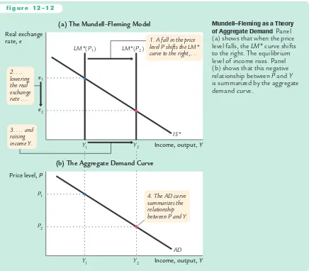
Figure 12-12 shows what happens when the price level falls. Because a lower
price level raises the level of real money balances, the LM* curve shifts to the
right, as in panel (a) of Figure 12-12.The real exchange rate depreciates, and the equilibrium level of income rises.The aggregate demand curve summarizes this negative relationship between the price level and the level of income, as shown in panel (b) of Figure 12-12.
Thus, just as the IS–LM model explains the aggregate demand curve in a
closed economy, the Mundell–Fleming model explains the aggregate demand
curve for a small open economy. In both cases, the aggregate demand curve shows the set of equilibria that arise as the price level varies. And in both cases, anything that changes the equilibrium for a given price level shifts the aggregate demand curve. Policies that raise income shift the aggregate demand curve to the right; policies that lower income shift the aggregate demand curve to the left.
f i g u r e 1 2 - 1 2
(b) The Aggregate Demand Curve
4. The AD curve level P shifts the LM* curve to the right, . . .
Mundell–Fleming as a Theory
of Aggregate Demand Panel
(a) shows that when the price
level falls, the LM*curve shifts
to the right. The equilibrium level of income rises. Panel (b) shows that this negative
relationship between Pand Y
We can use this diagram to show how the short-run model in this chapter is re-lated to the long-run model in Chapter 5. Figure 12-13 shows the short-run and long-run equilibria. In both panels of the figure, point K describes the short-run equilibrium, because it assumes a fixed price level.At this equilibrium, the demand for goods and services is too low to keep the economy producing at its natural rate. Over time, low demand causes the price level to fall.The fall in the price level raises real money balances, shifting the LM* curve to the right. The real exchange rate depreciates, so net exports rise. Eventually, the economy reaches point C, the long-run equilibrium. The speed of transition between the short-long-run and long-long-run equilibria depends on how quickly the price level adjusts to restore the economy to the natural rate.
(a) The Mundell–Fleming Model
(b) The Model of Aggregate Supply and Aggregate Demand Equilibria in a Small Open
Economy Point K in both panels
shows the equilibrium under the Keynesian assumption that the price level is fixed at P
1. Point C
concern in this chapter has been how policy influences point K, the short-run equilibrium. In Chapter 5 we examined the determinants of point C, the long-run equilibrium. Whenever policymakers consider any change in policy, they need to consider both the short-run and long-run effects of their decision.
12-7
A Concluding Reminder
In this chapter we have examined how a small open economy works in the short
run when prices are sticky.We have seen how monetary and fiscal policy influence
income and the exchange rate, and how the behavior of the economy depends on
whether the exchange rate is floating or fixed. In closing, it is worth repeating a
les-son from Chapter 5. Many countries, including the United States, are neither closed economies nor small open economies: they lie somewhere in between.
A large open economy, such as the United States, combines the behavior of a closed economy and the behavior of a small open economy.When analyzing poli-cies in a large open economy, we need to consider both the closed-economy logic of Chapter 11 and the open-economy logic developed in this chapter.The appendix to this chapter presents a model for a large open economy.The results of that model are, as one would guess, a mixture of the two polar cases we have already examined. To see how we can draw on the logic of both the closed and small open economies and apply these insights to the United States, consider how a mone-tary contraction affects the economy in the short run. In a closed economy, a monetary contraction raises the interest rate, lowers investment, and thus lowers
aggregate income. In a small open economy with a floating exchange rate, a
monetary contraction raises the exchange rate, lowers net exports, and thus low-ers aggregate income.The interest rate is unaffected, however, because it is
deter-mined by world financial markets.
The U.S. economy contains elements of both cases. Because the United States is large enough to affect the world interest rate and because capital is not perfectly mobile across countries, a monetary contraction does raise the interest rate and de-press investment. At the same time, a monetary contraction also raises the value of
the dollar, thereby depressing net exports. Hence, although the Mundell–Fleming
model does not precisely describe an economy like that of the United States, it does predict correctly what happens to international variables such as the exchange rate, and it shows how international interactions alter the effects of monetary and
fiscal policies.
Summary
1.The Mundell–Fleming model is the IS–LMmodel for a small open economy.
It takes the price level as given and then shows what causes fluctuations in
income and the exchange rate.